Biotech7005

Setup
NGS Data
Quality Control
Trimming and Quality Filtering of NGS data

Setup

Before we begin our material for today, we first need to set ourselves up like we have for most other weeks. Using the Terminal in RStudio, run the following commands.

cd
mkdir Practical_6

Once you have this setup, create a new R Project which can live in this directory. If you can’t remember how to do this, call a tutor over.

In addition, we’ve found that some software wasn’t installed as expected on your VMs. Please execute the following code. Hopefully it makes sense, but if not, ask a tutor. You will most likely encounter some messages asking for permission to update grub. Please answer yes or y as appropriate.

wget https://raw.githubusercontent.com/UofABioinformaticsHub/Biotech7005/master/updateVMs.sh
chmod +x updateVMs.sh
sudo ./updateVMs.sh

Also note that after you’ve entered that final line (beginning with sudo), you’ll need to enter your password.

NGS Data

Next generation sequencing (NGS) has become an important tool in assessing biological signal within an organism or population. Stemming from previous low throughput technologies that were costly and time-consuming to run, NGS platforms are relatively cheap and enable the investigation of the genome, transcriptome, methylome etc at extremely high resolution by sequencing large numbers of RNA/DNA fragments simultaneously. The high throughput of these machines also has unique challenges, and it is important that scientists are aware of the potential limitations of the platforms and the issues involved with the production of good quality data.

In this course, we will introduce the key file types used in genomic analyses, illustrate the fundamentals of Illumina NGS technology (the current market leader in the production of sequencing data), describe the affect that library preparation can have on downstream data, as well as running through a basic workflow used to analyse NGS data.

Before we can begin to explore any data, it is helpful to understand how it was generated. Whilst there are numerous platforms for generation of NGS data, today we will look at the Illumina Sequencing by Synthesis method, which is one of the most common methods in use today. Many of you will be familiar with the process involved, but it may be worth looking at the following 5-minute video from Illumina.

This video picks up after the process of fragmentation, as most strategies require DNA/RNA fragments within a certain size range. This step may vary depending on your experiment, but the important concept to note during sample preparation is that the DNA insert has multiple sequences ligated to either end. These include 1) the sequencing primers, 2) index and/or barcode sequences, and 3) the flow-cell binding oligos.

Barcodes vs Indexes

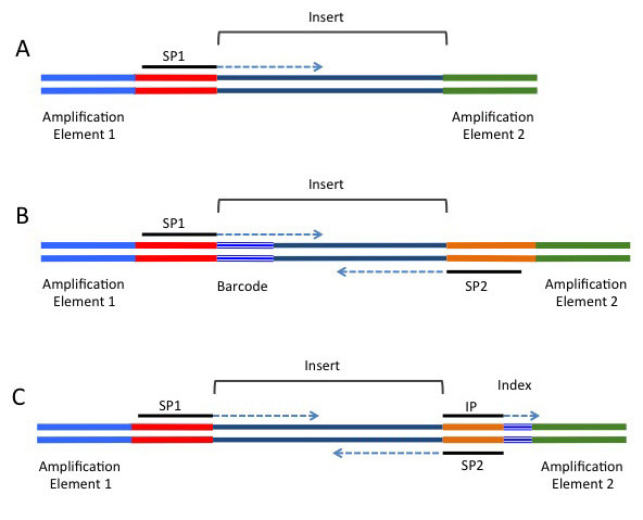
In the video, you may have noticed an index sequence being mentioned which was within the sequencing primers and adapters ligated to each fragment. Under this approach, a unique index is added to each sample during library preparation and these are used to identify which read came from which sample. This is a common strategy in RNA-Seq libraries and many other analyses with relatively low replicate numbers (i.e <= 16 transcriptomes). Importantly, the index will not be included in either the forward or reverse read.

A common alternative for analyses such as RAD-seq or GBS-seq, where population level data is being sequenced using a reduced representation approach. In these strategies, a barcode is added in-line and is directly next to the restriction site used to fragment the data (if a restriction enzyme approach was used for fragmentation). These barcodes are included next to the genomic sequence, and will be present in either or both the forward or reverse reads, depending on the barcoding strategy being used. A single barcode is shown in B) of the following image (taken from https://rnaseq.uoregon.edu/), whilst a single index is shown in C).

FASTQ File Format

As the sequences are extended during the sequencing reaction, an image is recorded which is effectively a movie or series of frames at which the addition of bases is recorded and detected. We mostly don’t deal with these image files, but will handle data generated from these in fastq format, which can commonly have the file suffix .fq or .fastq. As these files are often very large, they will often be zipped using gzip or bzip.
Whilst we would instinctively want to unzip these files using the command gunzip, most NGS tools are able to work with zipped fastq files, so decompression (or extraction) is not usually necessary. This can save considerable hard drive space, which is an important consideration when handling NGS datasets as the quantity of data can easily push your storage capacity to its limit.

The data for today’s practical has not yet been copied during the VM setup, so let’s get the files we need for today. This file may take a few moments to download if we all do this simultaneously, but hopefully it will work for all of you without too many issues.

Using the Terminal in RStudio, execute the following commands, paying special attention to upper and lower case characters. If you get these correct, all of today’s code should just work. If you don’t get these correct, you may end up being confused.

mkdir -p ~/Practical_6/0_rawData/fastq
cd ~/Practical_6/0_rawData/fastq
wget https://universityofadelaide.box.com/shared/static/0w0fgnm94w18ixh1z0dkmh5e0xht1ajf.gz -O multiplexed.tar.gz

Make sure you understand each of the above lines and discuss with your neighbour or a tutor if you’re confused.

Now we have downloaded the data, let’s:

extract (i.e. decompress) what we have (tar -xzvf)
remove the original file to save space (rm)
move one of the files we obtained to a convenient location. (mv)

tar -xzvf multiplexed.tar.gz
rm multiplexed.tar.gz
mv barcodes_R1.txt  ../../

The command zcat unzips a file and prints the output to the terminal, or standard output (stdout). If we did this to these files, we would see a stream of data whizzing past in the terminal, but instead we can just pipe the output of zcat to the command head just to view the first few lines of a file.

zcat Run1_R1.fastq.gz | head -n8

In the above command, we have used a trick commonly used in Linux systems where we have taken the output of one command (zcat Run1_R1.fastq.gz) and sent it to another command (head) by using the pipe symbol (|). This is literally like sticking a pipe on the end of a process and redirecting the output to the input another process (you should remember this from your Introduction to Bash Practicals).
Additionally, we gave the argument -n8 to the command head to ensure that we only printed the first eight lines.

This gives a clear view of the fastq file format, where each individual read spans four lines. These lines are:

The read identifier
The sequence of the read itself
An alternate line for the identifier (commonly left blank as just a + symbol acting as a placeholder)
The quality scores for each position along the read as a series of ASCII text characters. Let’s have a brief look at each of these lines and what they mean.

1. The read identifier

This line begins with an @ symbol and although there is some variability between different sequencing platforms and software versions, it traditionally has several components.
For the first sequence in this file, we have the full identifier @M02262:117:000000000-AMEE3:1:2105:14127:1629 1:N:0:CGACCTG which has the following components separated by colons (:)

`@M02262`	The unique machine ID. This line always begins with an `@` symbol
`117`	Run number
`000000000-AMEE3`	The flowcell ID
`1`	The flowcell lane
`2105`	The tile within the flowcell lane
`14127`	The x-coordinate of the cluster within the tile
`1629`	The y-coordinate of the cluster within the tile

After this we have a second colon-delimited field which contains the following information:

`1`	Indicates that this is the first read in a set of paired-end reads. This would be `2` for the second read in a pair
`N`	Indicated that this read was NOT marked as a bad quality read by Illumina’s own checks
`0`	Value indicating if a read is a control read (0 means it’s not)
`CGACCTG`	This was the index used when ligating adapters, as described above

As seen in the subsequent sections, these pieces of information can be helpful in identifying if any spatial effects have affected the quality of the reads. By and large you won’t need to utilise most of this information, but it can be handy for times of serious data exploration.

While we are inspecting our data, have a look at the beginning of the second file.

zcat Run1_R2.fastq.gz | head -n8

Here you will notice that the information in the identifier is identical to the first file we inspected, with the exception that there is a 2:N:0 at the beginning of the second component. This indicates that these reads are the second set in what are known as paired-end reads, as were introduced in the above video. The two files will have this identical structure where the order of the sequences in one is identical to the order of the sequences in the other. This way when they are read as a pair of files, they can be stepped through read-by-read and the integrity of the data will be kept intact. As you may recall, these paired reads are simply an initial fragment sequenced from one end, then from the other. Depending on the fragment size, they may or may not overlap in the middle.

Question

If we had 100bp paired-end reads, how short would a fragment have to be for the two reads to overlap?

2. The Sequence Read

Moving onto the second line, we get to the sequence read itself. This is a pretty obvious line, and just contains the sequence generated from each cluster on the flow-cell. Notice, that after this line is one which just begins with the + symbol and is blank. In early versions of the technology, this repeated the sequence identifier, but this is now just a placeholder.

3. Quality Scores

The only other line in the fastq format that really needs some introduction is the quality score information. These are presented as single ASCII text characters for simple visual alignment with the sequence. In the ASCII text system, each character has a numeric value which we can interpret as an integer, and in this context is the quailty score for the corresponding base. Head to the website with a description of these at ASCII Code table.

The first 31 ASCII characters are non-printable and contain things like end-of-line marks and tab spacings, and note that the first printable character after the space (character 32) is “!” which corresponds to the value 33. In short, the values 33-47 are symbols like !, #, $ etc, whereas the values 48-57 are the characters 0-9. Next are some more symbols (including @ for the value 64), with the upper case characters representing the values 65-90 and the lower case letters representing the values 97-122.

The PHRED +33/64 Scoring System

Now that we understand how to turn the quality scores from an ASCII character into a numeric value, we need to know what these numbers represent. The two main systems in common usage are PHRED +33 and PHRED +64 and for each of these coding systems we either subtract 33 or 64 from the numeric value associated with each ASCII character to give us a PHRED score. As will be discussed later, this score ranges between 0 and about 41.

The PHRED system used is determined by the software installed on the sequencing machine, with early machines using PHRED+64 (casava <1.5), and more recent machines tending to use PHRED+33.
For example, in PHRED+33, the @ symbol corresponds to Q = 64 - 33 = 31, whereas in PHRED +64 it corresponds to Q = 64 - 64 = 0.

The following table demonstrates the comparative coding scale for the different formats:

SSSSSSSSSSSSSSSSSSSSSSSSSSSSSSSSSSSSSSSSS.....................................................
..........................XXXXXXXXXXXXXXXXXXXXXXXXXXXXXXXXXXXXXXXXXXXXXX......................
...............................IIIIIIIIIIIIIIIIIIIIIIIIIIIIIIIIIIIIIIIII......................
.................................JJJJJJJJJJJJJJJJJJJJJJJJJJJJJJJJJJJJJJJ......................
LLLLLLLLLLLLLLLLLLLLLLLLLLLLLLLLLLLLLLLLLL....................................................
!"#$%&’()*+,-./0123456789:;<=>?@ABCDEFGHIJKLMNOPQRSTUVWXYZ[\]ˆ_‘abcdefghijklmnopqrstuvwxyz{|}~
|                         |    |        |                              |                     |
33                       59   64       73                             104                   126
S - Sanger Phred+33, raw reads typically (0, 40)
X - Solexa Solexa+64, raw reads typically (-5, 40)
I - Illumina 1.3+ Phred+64, raw reads typically (0, 40)
J - Illumina 1.5+ Phred+64, raw reads typically (3, 40)
L - Illumina 1.8+ Phred+33, raw reads typically (0, 41)

Interpretation of PHRED Scores

The quality scores are related to the probability of calling an incorrect base through the formula

Q = −10log₁₀P

where P is the probability of calling the incorrect base. This is more easily seen in the following table:

PHRED Score	Probability of Incorrect Base Call	Accuracy of Base Call
0	1 in 1	0%
10	1 in 10	90%
20	1 in 100	99%
30	1 in 1000	99.9%
40	1 in 10000	99.99%

Questions

Which coding system do you think has been used for the reads that we have?
In the PHRED +33 coding system, the character ‘@’ is used. Can you think of any potential issues this would cause when searching within a fastq file?
A common threshold for downstream inclusion of a sequence is a Q score >20. Considering the millions of sequences obtained from a flowcell, do you think that NGS is likely to be highly accurate?

Quality Control

Using FastQC

A common tool for checking the quality of a fastq file is the program FastQC. As with all programs on the command line, we need to see how it works before we use it. The following command will open the help file in the less pager which we used earlier. To navigate through the file, use the Spacebar to move forward a page, B to move back a page and Q to exit the manual.

fastqc -h | less

FastQC will create an html report for each file you provide, which can then be opened from any web browser such as firefox or chrome. As seen in the help page, FastQC can be run from the command line or from a graphic user interface (GUI). Using a GUI is generally intuitive but will be unavailable from our VMs, so today we will only look at the command line usage, as that will also give you more flexibility and options in the future. Some important options for the command can be seen in the manual. As you will see in the manual, setting the -h option as above will call the help page. Look up the following options to find what they mean.

Option	Usage
-o
-t

As we have two files, we will first need to create the output directory, then we can run fastqc using 2 threads which will ensure the files are processed in parallel. This can be much quicker when dealing with large experiments.

cd
mkdir ~/Practical_6/0_rawData/FastQC
fastqc -o ~/Practical_6/0_rawData/FastQC -t 2 ~/Practical_6/0_rawData/fastq/*gz

It’s probably a good idea to scribble a note next to each line if you didn’t understand what you did. If you haven’t seen the command mkdir before, check the help page man mkdir.

The above command:

Gave both files to fastqc using *gz. Note the use of the * wild-card here
Specified where to write the output (-o ~/Practical_6/0_rawData/FastQC) and
Requested two threads (-t 2).

Let’s see what we have:

cd ~/Practical_6/0_rawData/FastQC
ls -lh

The reports are in html files, which may be in the FastQC directory, or may be in the directories for the individual files, (depending on your version of FastQC). When working on your own data, you’ll find the html files then open using your favourite browser. As we’re already using RStudio to connect to our VM, use the Files pane to navigate to ~/Practical_6/0_rawData/FastQC and click on one of the html files you find. (If you don’t see any html files there call a tutor). Choose View in Web Browser and this file will open in your browser.

Inspecting a FastQC Report

The left hand menu contains a series of clickable links to navigate through the report, with a quick guideline about each section given as a tick, cross or exclamation mark.

Questions

How many sequences are there in both files?
How long are the sequences in these files?

Interpreting the FASTQC Report

As we work through the QC reports we will develop a series of criteria for filtering and cleaning up our files. There is usually no perfect solution, we just have to make the best decisions we can based on the information we have. Some sections will prove more informative than others, and some will only be helpful if we are drilling deeply into our data. Firstly we’ll just look at a selection of the plots. We’ll investigate some of the others with some ‘bad’ data later.

Per Base Sequence Quality

Both of the files should be open in firefox in separate tabs. Perform the following steps on both files. Click on the Per base sequence quality hyper-link on the left of the page and you will see a boxplot of the QC score distributions for every position in the read. This is the first plot that bioinformaticians will look at for making informed decisions about later stages of the analysis.

What do you notice about the QC scores as you progress through the read?

We will deal with trimming the reads in a later section, but start to think about what you should do to the reads to ensure the highest quality in your final alignment and analysis.

Per Tile Sequence Quality This section just gives a quick visualisation about any physical effects on sequence quality due to the tile within the each flowcell or lane. Most of the time we don’t use this plot for many trimming or filtering decisions, however it can alert us to any problems with the flow cell, or camera, or if there’s been a blockage in the lane. If we see clear spatial effects, we may think about contacting the sequence provider for a repeat run of our material.

Per Sequence Quality Scores This is just the distribution of average quality scores for each sequence. There’s not much of note for us to see here.

Per Base Sequence Content This will often show artefacts from barcode sequences or adapters early in the reads, before stabilising to show a relatively even distribution of the bases.

Sequence Length Distribution This shows the distributions of sequence lengths in our data. Here we have sequences that are all the same lengths, however if the length of your reads is vital (e.g. smallRNA data), then this can also be an informative plot.

Sequence Duplication Levels This plot shows about what you’d expect from a typical NGS experiment. There are few to no duplicated sequences (rRNA, highly expressed genes etc.) and lots of unique sequences represented the diverse transcriptome. This is only calculated on a small sample of the library for computational efficiency and is just to give a rough guide if anything unusual stands out.

Overrepresented Sequences Here we can see any sequence which are more abundant than would be expected. Sometimes you’ll see sequences here that match the adapters used, or you may see highly expressed genes here.

Adapter Content This can give a good guide as to our true fragment lengths. If we have read lengths which are longer than our original DNA/RNA fragments (i.e. inserts) then the sequencing will run into the adapters. If you have used custom adapters, you may need to supply them to FastQC as this only searches for common adapter sequences.

Some More Example Reports

Let’s head to another sample plot at the FastQC homepage

Per Base Sequence Quality Looking at the first plot, we can clearly see this data is not as high quality as the one we have been exploring ourselves.

Per Tile Sequence Quality Some physical artefacts are visible and some tiles seem to be consistently lower quality. Whichever approach we take to cleaning the data will more than likely account for any of these artefacts. Sometimes it’s just helpful to know where a problem has arisen.

Overrepresented Sequences Head to this section of the report and scan down the list. Unlike our sample data, there seem to be a lot of enriched sequences of unknown origin. There is one hit to an Illumina adapter sequence, so we know at least one of the contaminants in the data. Note that some of these sequences are the same as others on the list, just shifted one or two base pairs. A possible source of this may have been non-random fragmentation.

Interpreting the various sections of the report can take time and experience. A description of each of the sections is available from the fastqc authors which can be very helpful as you’re finding your way.

Another interesting report is available at http://www.bioinformatics.babraham.ac.uk/projects/fastqc/RNA-Seq_fastqc.html. Whilst the quality scores generally look pretty good for this one, see if you can find a point of interest in this data. This is a good example, of why just skimming the first plot may not be such a good idea.

Working With Larger Datasets

In our dataset of two samples it is quite easy to think about the whole experiment and assess the overall quality.

What about if we had 100 samples?

Each .zip archive contains text files with the information which can easily be parsed into an overall summary. We could write a script to extract this information if we had the time. However, some members of the Bioinformatics Hub have published an R package to help with this, which is available from https://bioconductor.org/packages/release/bioc/html/ngsReports.html and is installed on your VM already. It won’t be too useful today, but may be useful in the future.

Trimming and Quality Filtering of NGS data

Once we have inspected our data and have an idea of how accurate our reads are, as well as any other technical issues that may be within the data, we may need to trim adapter sequences or filter the reads to make sure we are aligning or analysing sequences that accurately represent our source material.
As we’ve noticed, the quality of reads commonly drops off towards the end of the reads, and dealing with this behaviour is an important part of most processing pipelines. Sometimes we will require reads of identical lengths for our downstream analysis, whilst other times we can use reads of varying lengths. The data cleaning steps we choose for our own analysis will inevitably be influenced by our downstream requirements.

The Basic Workflow

Data cleaning and pre-processing can involve many steps, and today we will use the basic work-flow as outlined below. Every analysis is slightly different so some steps may or may not be required for your own data. Some steps do have a little overlap, and some pipelines may perform some of these steps for you.

Using today’s dataset, we will take one sequencing experiment through de-multiplexing and adapter removal. We will perform most steps on files at this stage, rather than on a complete library, but the principle is essentially the same.

A basic workflow is:

Remove Low Quality Reads (fastq_illumina_filter). This wil usually not be required on recent datasets, and is only required if you see reads with 1:Y:0 or 2:Y:0 in the sequence headers. These reads have now been excluded by sequence providers for the last few years.
Remove Adapters (cutadapt or Adapter Removal)
Remove Low Quality Bases. This is usually done by our adapter removal tools whilst trimming, and can be performed by trimming:
1. based on quality scores
2. to a fixed length
Demultiplexing (sabre, fastq_multx or process_radtags).
Alignment to a reference (bwa, bowtie2, STAR)
Post-alignment QC (picard markDuplicates, IGV)

Removal of Low Quality Reads and Adapters

Adapter removal is an important step in many sequencing projects, mainly projects associated with small DNA/RNA inserts. For example, a common RNAseq experiment is to sequence small non-coding RNAs that are generated by an individual to regulate other coding sequences. These small RNAs (namely miRNAs, snoRNAs and/or siRNAs) are generally between 19-35bp, which is significantly smaller than the shortest, standard read length of most Illumina MiSeq/NextSeq/HiSeq machines (usually have read length settings such as 50, 75, 100, 125, 250 or 300bp). Therefore it is important to trim adapters accurately to ensure that the genome mapping and other downstream analyses are accurate.

Previously we would run multiple steps to remove both low-quality reads, but today’s trimming algorithms have become better at removing low-quality data and the same time as removing adapters. The tool we’ll use today is cutadapt and it’s one of the few bioinformatics tools to have a helpful web page, so head to the site.

Now we can trim the raw data using the Illumina TruSeq paired-end adapters obtained from this website These are commonly used in Illumina projects.

Before we perform adapter trimming, look at the following code.

cd ~/Practical_6
mkdir -p 1_trimmedData/fastq
mkdir -p 1_trimmedData/FastQC
mkdir -p 1_trimmedData/log
cutadapt \
	-m 35 \
	-q 20 \
	-a AGATCGGAAGAGCACACGTCTGAAC \
	-A AGATCGGAAGAGCGTCGTGTAGGGA \
	-o 1_trimmedData/fastq/Run1_R1.fastq.gz \
	-p 1_trimmedData/fastq/Run1_R2.fastq.gz \
	0_rawData/fastq/Run1_R1.fastq.gz 0_rawData/fastq/Run1_R2.fastq.gz > \
	1_trimmedData/log/cutadapt.log

Note that the symbol \ has been included at the end of some of these lines. This is often used in a script to break a long command over multiple lines to make it easier to read. Notice how by using this technique, it’s very easy to see every parameter and argument that has been set when we run cutadapt.

Another point worth making is how we’ve created the directory structure. NGS data analysis often requires multiple steps and keeping every step well organised can be extremely helpful for finding your way around later. Although this may appear trivial, in the real world decisions you make at this point can become quite significant. Poor decisions can lead to accidental file deletions and general difficulties just finding where everything is.

Questions

1. What do the settings -m 35 and q 20 do in the above? 2. Why have we specified sequences using -a and -A?

If we ran the above code by cutting and pasting, we would successfully trim the pair of reads Run1_R1.fastq.gz and Run1_R2.fastq.gz which we have placed in the folder 0_rawData/fastq. During this process, the cutadapt tool produces a large amount of information about the trimming process. In the above we would write this output to a log file using the > symbol to redirect stdout to a file. Let’s have a look in the file to check the output.

less cutadapt.log

As these were a good initial sample, it’s not surprising that we didn’t lose many sequences. Notice that many reads were trimmed, but were still long enough and high enough quality to be retained.

Note the spread of A/C/G/T bases which appeared before the adapter sequences. This can indicates if we’ve missed anything, as sometimes you’ll see a strong bias in the last base before the adapter.

FastQC

Before moving on, we need to check the quality of the trimmed sequences, so let’s run fastqc on these files to check them out. Make sure you’re in the correct directory first!

mkdir -p 1_trimmedData/FastQC
fastqc -o 1_trimmedData/FastQC -t 2 1_trimmedData/fastq/*gz

Question

Was there much of an improvement in the trimmed data?

Demultiplexing

In the first section we discussed the difference between an index and a barcode. If you use an indexed adapter to distinguish samples on an Illumina sequencing run, the de-multiplexing is usually done on the sequencing machine. However, sometimes it makes sense to use a barcode (or sometimes called “in-line barcode”), to further multiplex samples onto one sequencing run.

While barcodes can be incredibly useful, it is important to note that Illumina cycle calibration and cluster calling is done in the first 4 cycles (first four base-pairs of read 1). It also is used to establish other metrics (e.g., signal thresholds) for base-calling. Therefore it is essential that the first four base pairs are “diverse” (i.e. no particular nucleotide is over-represented in the first four base-pairs). Designing the right barcodes to add to the start of your reads extremely important!

Our samples today have a 7bp barcode at the start of the reads. We can see these pretty clearly with a little usage of our newly learned bash skills.

zcat 1_trimmedData/fastq/Run1_R1.fastq.gz | sed -n '2~4p' | cut -c 1-7 | sort | uniq -c | sort -n -r | head

The command above is quite long and contains multiple bash commands that are separated by a pipe. What does each command do?

Command	Explanation
`zcat Run1_R1.fastq.gz`	Prints the compressed fastq file to screen
`sed -n '2~4p'`	Prints the second line (sequence of each fastq file)
`cut -c 1-7`	Get the first 7 characters
`sort`	sort the sequences
`uniq -c`	Find the unique sequences are count them
`sort -n -r`	sort the sequences numerically and reverse the order
`head`	Print the top 10

Notice that two particular sequences are highly abundant, whilst the rest are just noise, or variations on the barcodes with sequencing errors. The two barcodes match those give in the file barcodes_R1.txt which we moved at the start of the session. Our barcode sequences should be “GCGTAGT” (for the sample bc1) and “CCTCGTA” (for the sample bc2). You can check this using cat barcodes_R1.txt

To demultiplex, we’ll use a tool called sabre. Unfortunately, sabre only runs with uncompressed data, so to run this program we’ll need to unzip our fastq files.

cd 1_trimmedData/fastq
gunzip Run1_R*

Now we’ve successfully performed this step, we can run sabre. Before we run this let’s check the help page

sabre --help

If you ask us, this isn’t helpful and this is a common problem with tools for NGS data. As we’re going to to be using this tool in paired-end mode we can find the help we need using

sabre pe --help

Many NGS (and other) tools use this strategy of having a sub-command following the main command which tells the main tool (sabre) to operate in a specific stage or mode (pe). We can then call the specific help page for this mode.

cd ~/Practical_6
mkdir -p 2_demultiplexedData/fastq
cd 2_demultiplexedData/fastq
sabre pe \
	-m 1 \
	-f ../../1_trimmedData/fastq/Run1_R1.fastq \
	-r ../../1_trimmedData/fastq/Run1_R2.fastq \
	-b ../../barcodes_R1.txt \
	-u unknown_R1.fastq \
	-w unknown_R2.fastq 

How many read pairs were extracted in each sample? Does this match the number we found by grabbing out the first 7 bases in bash?

Run the command again without the one mismatch. How many read are now in each?

Note the clear directory structure that we’ve used. This can lead to a command that is tricky to understand at first, but try to keep track of the file paths. Why do you think we might use this particular file structure? In a real-world context, we’d probably script this too so file paths may be declared as variables.

Writing an actual script

In the above example, we just ran all tools from the terminal. This would not be reproducible as we have no record of this process. We should keep everything as a script so we could run the entire workflow as a single script.

In RStudio open a new plain text file: File > New File > Text File. Save this in your ~/Practical_6 folder as runPipeline.sh. Notice that RStudio seems to recognise this as a bash script and will add a little icon to the top of your file.

At the beginning of this file, add the shebang:

#!/bin/bash

Leaving a blank line after the shebang, copy and paste the following code into this script:

PROJROOT=/home/biotech7005/Practical_6
RAWDIR=${PROJROOT}/0_rawData

# Check the project root has been defined correctly
if [[ ! -d ${PROJROOT} ]]; then
	echo -e "Couldn't find ${PROJROOT}\n. Exiting now"
	exit 1
fi 

# Make sure we have a directory for FastQC output, then run it
if [[ ! -d ${RAWDIR}/FastQC ]]; then
	mkdir -p ${RAWDIR}/FastQC
fi
fastqc -o ${RAWDIR}/FastQC -t 2 ${RAWDIR}/fastq/*gz

This is exactly how we do things in the real world of bioinformatics. Note that we defined our main project folder as the variable PROJROOT, then checked for the presence of this folder, exiting quickly and informatively if it doesn’t exist.

We then became exceedingly lazy and didn’t check for the presence of any raw data. How would we do this?

After initial checks, we then checked for the directory ${RAWDIR}/FastQC and created it if it didn’t already exist. Now we know that our output directory exists, we can fun fastqc. Notice here that we’ve been reusing the variable RAWDIR quite a few times, showing you just how handy this trick is.

Save the script and make it executable using chmod +x runPipeline.sh. Once you’ve done this, try running it using ./runPipeline.sh, ensuring you are in the correct folder first. Now we can repeat this process any time with great ease and for any new dataset, we just need to change the initial file paths and could run this for this new (but imaginary) dataset. Hopefully now you’ll see some of the usefulness of our strategies here.

See if you can build a complete script to run today’s pipeline, including running fastqc on our demultiplexed data! After our initial code you’ll need to run cutadapt making sure you check and define directories, followed by fastqc on the trimmed data. Then you’ll need to unzip the trimmed files, demultiplex and run fastqc. If you’re keen, you could also try gzipping the trimmed data again after you’ve demultiplexed.