Introduction to NGS Data
![]()
Course Homepage
September 2017
This project is maintained by UofABioinformaticsHub
NGS Data Generation
Before we can begin to analyse any data, it is helpful to understand how it was generated. Whilst there are numerous platforms for generation of NGS data, today we will look at the Illumina Sequencing by Synthesis method, which is one of the most common methods in use today. Many of you will be familiar with the process involved, but it may be worth looking at the following 5-minute video from Illumina:. As setting up the sound with the VMs can be tricky, it will be easier to view this from your own regular browser. Briefly minimise the VM (see Section 1.4), open your regular browser & please use your headphones if you brought them.
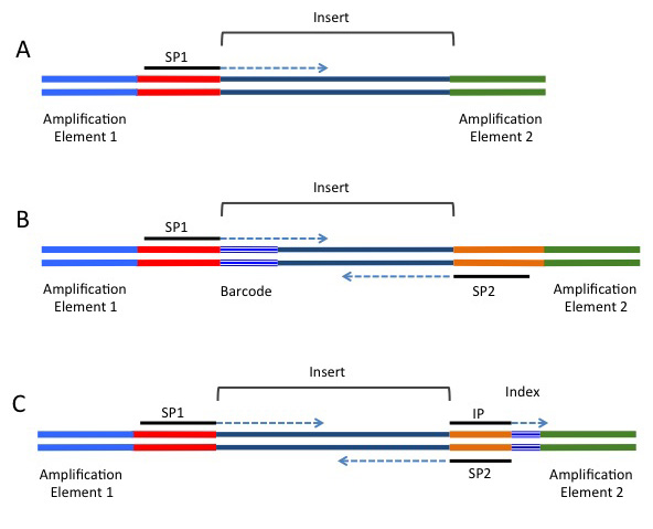
This video refers to the process tagmentation. This is a relatively recent method for fragmenting & attaching adapters to DNA, with an alternative, more traditional methods being sonication, poly-adenylation & attachment of appropriate adaptors in separate steps. This step may vary depending on your experiment, but the important concept to note during sample preparation is that the DNA insert has multiple sequences ligated to either end. These include 1) the sequencing primers, 2) index & /or barcode sequences, and 3) the flow-cell binding oligos. To demonstrate these concepts further, observe the following figure that shows the DNA construct needed to run an illumina sequencing run, and the amplification steps required:
FASTQ File Format
As the sequences are extended during the sequencing reaction, an image is recorded which is effectively a movie or series of frames at which the addition of bases is recorded & detected. We mostly don’t deal with these image files, but will handle data generated from these in fastq format, which can commonly have the file suffix .fq or .fastq. As these files are often very large, they will often be zipped using gzip or bzip. Whilst we would instinctively want to unzip these files using the command gunzip, most NGS tools are able to work with zipped fastq files, so decompression (or extraction) is usually unnecessary. This can save considerable hard drive space, which is an important consideration when handling NGS datasets as the quantity of data can easily push your storage capacity to it’s limit.
We should still have a terminal open from the previous section &, if necessary, use the cd command to make sure you are in the home (~/) directory. The command zcat unzips a file & prints the output to the terminal, or standard output (stdout). If we did this to these files, we would see a stream of data whizzing past in the terminal, but instead we can just pipe the output of zcat to the command head to view the first 10 lines of a file.
cd ~/WGS/rawData/fastq
zcat SRR2003569_sub_1.fastq.gz | head -n8
In the above command, we have used a trick commonly used in Linux systems where we have taken the output of one command (zcat SRR2003569_sub_1.fastq.gz) and sent it to another command (head) by using the pipe symbol (|). This is literally like sticking a pipe on the end of a process & redirecting the output to the input another process. If you think of things as being like a data factory you can almost visualise it. There are no limits to the number of commands that you can string together using this trick. Additionally, we gave the argument -n8 to the command head to ensure that we only printed the first eight lines.
In the output from the above terminal command, we have obtained the first 8 lines of the gzipped fastq file. This gives a clear view of the fastq file format, where each individual read spans four lines. These lines are:
- The read identifier
- The sequence read
- An alternate line for the identifier (commonly left blank as just a + symbol acting as a placeholder)
- The quality scores for each position along the read as a series of ascii text characters. Let’s have a brief look at each of these lines and what they mean.
The read identifier
This line begins with an @ symbol and although there is some variability, it traditionally has several components. Today’s data have been sourced from an EBI data repository with the identifier SRR065388. For the first sequence in this file, we have the full identifier @SRR2003569.1 JLK5VL1:245:D1DF6ACXX:6:1101:4181:2239/1 which has the following components:
| @SRR2003569.1 | The aforementioned EBI identifier & the sequence ID within the file. As this is the first read, we have the number 1. NB: This identifier is not present when data is obtained directly from the machine or service provider. |
| JLK5VL1:245:D1DF6ACXX | The unique machine ID |
| 6 | The flowcell lane |
| 1101 | The tile within the flowcell lane |
| 4181 | The x-coordinate of the cluster within the tile |
| 2239 | The y-coordinate of the cluster within the tile |
| /1 | Indicates that this is the first read in a set of paired-end reads |
As seen in the subsequent sections, these pieces of information can be helpful in identifying if any spatial effects have affected the quality of the reads. By and large you won’t need to utilise most of this information, but it can be handy for times of serious data exploration.
While we are inspecting our data, have a look at the beginning of the second file.
zcat SRR2003569_sub_2.fastq.gz | head -n8
Here you will notice that the information in the identifier is identical to the first file we inspected, with the exception that there is a /2 at the end. This indicates that these reads are the second set in what are known as paired-end reads, as were introduced in the above video. The two files will have this identical structure where the order of the sequences in one is identical to the order of the sequences in the other. This way when they are read as a pair of files, they can be stepped through read-by-read & the integrity of the data will be kept intact.
The Illumina Chastity Filter
It is also worth noting that the reads we’ve just glanced at come from a version of the Illumina casava pipeline which is <1.8, and which is a relatively common format. The casava version really just describes how old the software on the Illumina machine is & we don’t choose this. For more recently generated reads where the casava software is >1.8 of the casava, there is an additional field in the identifier which indicates whether a read would have failed an initial QC check. An example of this format would be:
@D5B4KKQ1:554:C4YHPACXX:4:1101:1084:2100 1:Y:0:
Note the “Y” in the final fields, which indicates this sequence would have failed QC.
These low-quality reads were automatically removed in earlier versions of the pipeline and were omitted from the fastq file.
However, they are now included by some sequence providers with this additional field indicated in the read identifier.
Inspection of this line will enable you to find out which version of the casava pipeline has been used, and whether you need to perform any additional filtering steps to remove low quality reads.
The tool fastq illumina filter is designed to remove these reads for you & the tool, along with usage instructions.
We won’t spend any further time on this today, but it can be an important thing to be aware of.
Quality Scores
The only other line in the fastq format that really needs some introduction is the quality score information. These are presented as single ascii text characters for simple visual alignment with the sequence, and each character corresponds to a numeric value, which is the quality score. In the ascii text system, each character has a numeric value which we can interpret as an integer. Head to the website with a description of these at ASCII Code table.
The first 31 ASCII characters are non-printable & contain things like end-of-line marks and tab spacings, and note that the first printable character after the space (character 32) is “!” which corresponds to the value 33. In short, the values 33-47 are symbols like !, #, $ etc, whereas the values 48-57 are the characters 0-9. Next are some more symbols (including @ for the value 64), with the upper case characters representing the values 65-90 & the lower case letters representing the values 97-122.
The PHRED +33/64 Scoring System
Now that we understand how to turn the quality scores from an ascii character into a numeric value, we need to know what these numbers represent. The two main systems in common usage are PHRED +33 and PHRED +64 and for each of these coding systems we either subtract 33 or 64 from the numeric value associated with each ascii character to give us a PHRED score. As will be discussed later, this score ranges between 0 and about 41.
The PHRED system used is determined by the software installed on the sequencing machine, with early machines using PHRED + 64 (casava <1.5), and more recent machines tending to use PHRED + 33. For example, in PHRED +33, the @ symbol corresponds to Q = 64 - 33 = 31, whereas in PHRED +64 it corresponds to Q = 64 - 64 = 0.
The following table demonstrates the comparative coding scale for the different formats:
SSSSSSSSSSSSSSSSSSSSSSSSSSSSSSSSSSSSSSSSS.....................................................
..........................XXXXXXXXXXXXXXXXXXXXXXXXXXXXXXXXXXXXXXXXXXXXXX......................
...............................IIIIIIIIIIIIIIIIIIIIIIIIIIIIIIIIIIIIIIIII......................
.................................JJJJJJJJJJJJJJJJJJJJJJJJJJJJJJJJJJJJJJJ......................
LLLLLLLLLLLLLLLLLLLLLLLLLLLLLLLLLLLLLLLLLL....................................................
!"#$%&’()*+,-./0123456789:;<=>?@ABCDEFGHIJKLMNOPQRSTUVWXYZ[\]ˆ_‘abcdefghijklmnopqrstuvwxyz{|}~
|                         |    |        |                              |                     |
33                       59   64       73                             104                   126
S - Sanger Phred+33, raw reads typically (0, 40)
X - Solexa Solexa+64, raw reads typically (-5, 40)
I - Illumina 1.3+ Phred+64, raw reads typically (0, 40)
J - Illumina 1.5+ Phred+64, raw reads typically (3, 40)
L - Illumina 1.8+ Phred+33, raw reads typically (0, 41)
Interpretation of PHRED Scores
The quality scores are related to the probability of calling an incorrect base through the formula
Q = −10log10P
where P is the probability of calling the incorrect base. This is more easily seen in the following table:
| PHRED Score | Probability of Incorrect Base Call | Accuracy of Base Call |
|---|---|---|
| 0 | 1 in 1 | 0% |
| 10 | 1 in 10 | 90% |
| 20 | 1 in 100 | 99% |
| 30 | 1 in 1000 | 99.9% |
| 40 | 1 in 10000 | 99.99% |
Questions
- Which coding system do you think has been used for the RNA-Seq reads that we have?
- In the PHRED +33 coding system, the character ‘@’ is used. Can you think of any potential issues this would cause when searching within a fastq file? 3.A common threshold for inclusion of a sequence is a Q score >20. Considering the millions of sequences obtained from a flowcell, do you think that NGS is likely to be highly accurate?