• NGS Data Generation
  • Barcodes vs Indexes
  • FASTQ File Format
    • Today’s RNA Seq Data
    • Introducing the FASTQ format
  • The Phred+33/64 Scoring Systems

NGS Data Generation

Before we can begin to analyse any data, it is helpful to understand how it was generated. while there are numerous platforms for generation of NGS data, today we will look at the Illumina Sequencing by Synthesis method, which is one of the most common methods in use today. Many of you will be familiar with the process involved, but it may be worth looking at the following 5-minute video from Illumina:.

This video picks up after the process of fragmentation, as most strategies require DNA/RNA fragments within a certain size range. This step may vary depending on your experiment, but the important concept to note during sample preparation is that the DNA insert has multiple oligonucleotide sequences ligated to either end. These include 1) the sequencing primers, 2) index and /or barcode sequences, and 3) the flow-cell binding oligos.

Illumina have released multiple sequencing machines, with a common platform being the various models of the NextSeq. Flow cells for the NextSeq models have four lanes, which are drawn from a common sample reservoir and are essentially a form of technical replicates. Example run times and yields for the Nextseq 550 High-Output Kit are given below:

Read Length	Total Time	Output	Yield
2 × 150 bp	29 hrs	100–120 Gb	< 800million
2 × 75 bp	18 hrs	50–60 Gb	< 800million
1 × 75 bp	11 hrs	25–30 Gb	< 400million

Note that for paired and single-end reads, the yield appears quite different. Importantly, the same number of fragments are sequenced, with the difference being that reads are generated in a single direction only, or with the additional sequencing from the opposite end of the fragment. Illumina also consider that a single flow cell is suitable for a single genome, 12 exomes or 16 transcriptomes, based on the size of the human genome.

Illumina have a comparison table for the different platforms and their uses.

Barcodes vs Indexes

In the video we watched earlier, you may have noticed an index sequence being discussed, which was within the sequencing primers and adapters ligated to each fragment. Under the approach they detailed, a unique index is added to each sample during library preparation and these are used to identify which read came from which sample. This is a common strategy in RNA-Seq libraries and many other analyses with relatively low replicate numbers (i.e <= 16 transcriptomes). Importantly, the index will not be included in either the forward or reverse read but is read as a separate step.

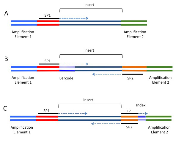
A common alternative for analyses such as RAD-seq or GBS-seq, where population level data is being sequenced using a reduced representation approach, and which commonly involves hundreds of samples. In these strategies, a barcode is added in-line and is directly next to the restriction site used to fragment the data (if a restriction enzyme approach was used for fragmentation). These barcodes are included next to the genomic sequence, and will be present in either (or both) of the forward or reverse reads, depending on the barcoding strategy being used. A single barcode is shown in B) of the following image (taken from https://rnaseq.uoregon.edu/), while a single index is shown in C).

FASTQ File Format

As the sequences are extended during the sequencing reaction, an image is recorded which is effectively a movie or series of frames at which the addition of bases is recorded and detected. We mostly don’t deal with these image files, but will handle data generated from these in FASTQ format, which can commonly have the file suffix .fq or .fastq. As these files are often very large, they will often be zipped using gzip or bzip. while we would instinctively want to unzip these files using the command gunzip, most NGS tools are able to work with zipped FASTQ files, so decompression (or extraction) is usually unnecessary. This can save considerable hard drive space, which is an important consideration when handling NGS datasets, as the quantity of data can easily push your storage capacity to it’s limit.

We should still have a terminal open from the previous section so ensure you have one open if you don’t. If necessary, use the cd command to make sure you are in the home (~/) directory.

Today’s RNA Seq Data

The data we are going to work with today is the folder ~/data, so let’s see what we have to start with.

ll -h data

The specific dataset we’ll start with is in the directory ~/data/aging_study, so let’s see what files are included.

ll -h data/aging_study

Here you should see output that looks like the following:

total 649M
drwxr-xr-x 2 trainee trainee 4.0K Apr 12 04:57 ./
drwxrwxr-x 3 trainee trainee 4.0K Apr 12 04:28 ../
-rw-r--r-- 1 trainee trainee 136M Apr 12 04:08 1_non_mutant_Q96_K97del_6mth_10_03_2016_S1_fem_R1.fq.gz
-rw-r--r-- 1 trainee trainee 124M Apr 12 04:08 2_non_mutant_Q96_K97del_6mth_10_03_2016_S2_fem_R1.fq.gz
-rw-r--r-- 1 trainee trainee 135M Apr 12 04:08 3_non_mutant_Q96_K97del_6mth_10_03_2016_S3_fem_R1.fq.gz
-rw-r--r-- 1 trainee trainee  57M Apr 12 04:57 4_non_mutant_Q96_K97del_24mth_23_04_2014_S1_fem_R1.fq.gz
-rw-r--r-- 1 trainee trainee  63M Apr 12 04:57 5_non_mutant_Q96_K97del_24mth_23_04_2014_S2_fem_R1.fq.gz
-rw-r--r-- 1 trainee trainee  74M Apr 12 04:57 6_non_mutant_Q96_K97del_24mth_23_04_2014_S3_fem_R1.fq.gz
-rw-r--r-- 1 trainee trainee  64M Apr 12 04:57 7_non_mutant_Q96_K97del_24mth_23_04_2014_S4_fem_R1.fq.gz

What did the -h flag do in the above commands?

Here we have 6 files with horribly long names, which is actually quite common in bioinformatics, but are actually very informative. For those interested, we are looking at the wild type (non_mutant) samples from a larger comparison with a mutant (Q96K97del), at two timepoints (6/26 months). All samples are zebrafish and the dates of sample preparation were in March 2014 or 2016. These are all taken from female fish, and we will only use the R1 reads, which is from the first round of sequencing as discussed in the video we watched earlier. Fortunately Tab auto-complete will make our lives easier when faced with these types of filenames.

Introducing the FASTQ format

The suffix given to all of the files above is fq.gz and this tells us that we (probably) have a compressed (using gzip compression) fastq file. You will often see them with either the fq.gz or fastq.gz combination.

Fortunately, we don’t need to decompress (or extract) these files as most NGS tools accept gz-compressed fastq files as input. To inspect a plain-text file, we saw the cat command yesterday, which dumped the entire contents of a file onto the stdout data stream. For compressed files, the command zcat will do the same thing, extracting the data before presenting it to stdout. Clearly, we have big files here and that information dump may take a while. Instead, we’ll just pipe that output into head, stopping after the first 8 lines.

(Remember to use Tab auto-complete instead of typing that huge filename!)

cd ~/data/aging_study
zcat 1_non_mutant_Q96_K97del_6mth_10_03_2016_S1_fem_R1.fq.gz | head -n8

This should give you the following, but please note that some lines may be wrapping around inside your terminal.

@NB501008:59:HVG7JBGXY:1:11101:10752:1058 1:N:0:AGCATCAC
CCTGATTTGAGTCATTGTGGTTTAGGCAATACTATCTGGCTAAAACTATACTTGACTATTGTGATAGTGTGTTCAGAAAACCCTGCTAATAAAGTACACAATGTTGTCACGTCATACGTACAAAACACTACAATTGTAATAACAAAAAAC
+
AAAAAEEEEEEEEEEEEEEEEEEEEEEEEEEEEEEEEEEEEEEEEEEEEEEEEEEEEEEEEEEEEEEEEEEEEEEEEEEEEEAEEEEEEEEEEEEEEEEEEEEEEEEAEEEEEEEEEEEEEEEEEEEEEEEAAEEAAEEEEEEAEEEEE<
@NB501008:59:HVG7JBGXY:1:11101:5594:1065 1:N:0:AGCATCAC
CAAAAATCCTTCATGAAAAAATATTCCAAAACTAAATATTTCACATAAACACATATTTGCCACATGAATTTCCGGCACAGGGATTTTGAGATCGGAAGAGCACACGTCTGAACTCCAGTCACAGCATCACATCTCGTATGCCGTCTTCTG
+
AAAAAEEEEEEEEEEEEEEEEEEEEEEEEEEEEEEEEEEEEEEEEEAEEEEEEEEEEAEEE<EEEEEEEEEEEAEA<EEEEEEEEEEEEEEEEEEAEEEEEAEAEEEEEEE/EEA/EEEEEEEEAAEEAAA/AAAEEAEEAAEE/EEEE<

In this output, we have obtained the first 8 lines of the gzipped FASTQ file. This gives a clear view of the FASTQ file format, where each individual read spans four lines. These four lines are:

1. The read identifier
2. The sequence read
3. An alternative line for the identifier (commonly left blank as just a + symbol acting as a placeholder)
4. The quality scores for each position along the read as a series of ASCII text characters.

In the above we have obtained 8 lines, thus we have all the information from two reads. Let’s have a brief look at each of these lines and what they mean.

1. The read identifier

This line begins with an @ symbol and although there is some variability between different sequencing platforms and software versions, it traditionally has several components. For the first sequence in this file, we have the full identifier @NB501008:59:HVG7JBGXY:1:11101:10752:1058 1:N:0:AGCATCAC which has the following components:

@NB501008	This is the ID for the sequencing machine
59	The run ID
HVG7JBGXY	The flowcell ID
1	The flowcell lane
11101	The tile within the flowcell lane
10752	The x-coordinate of the cluster within the tile
1058	The y-coordinate of the cluster within the tile
1	Indicates that this is the first read (1) out of any possible paired reads
N	The read has not been flagged as low quality by Illumina’s initial QC
0	Control bit (rarely used)
AGCATCAC	The barcode attached to this read

As seen in the subsequent sections, these pieces of information can be helpful in identifying if any spatial effects have impacted the quality of the reads. By and large you won’t need to utilise most of this information, but it can be handy for times of serious data exploration.

Whilst we won’t use paired reads today, it’s important to note that any corresponding R2 file that matches an R1 file will have the read taken from the other end of the initial fragments in exactly the same order as the R1 file. Logically, the identifier from an R2 file would be identical with the exception of the 1:N:0 triplet, which would likely become 2:N:0, assuming that the R2 passed Illumina’s initial QC. None of the other pieces of information would change.

This structure is often checked by tools as they perform their tasks, and it may be worth noting that Dropbox regularly fails to correctly sync files and as a result breaks this parallel structure with monotonous regularity. You might have to trust us on that one. Or you could learn the hard way…

2. The Sequence Read

The next line is pretty obvious, and just contains the actual sequence generated from each cluster on the flow-cell. Notice, that after this line is one which just begins with the + symbol and is blank. In early versions of the technology, this repeated the sequence identifier, but this is now just a placeholder.

3. Quality Scores

The only other line in the FASTQ format that really needs some introduction is the quality score information. These are presented as single ASCII text characters for simple visual alignment with the sequence.

A significant difference between FASTA and FASTQ is that FASTQ files contain information describing the confidence that can be placed on each base of the sequence, represented as a “Phred” score. In raw reads this is a measure of the confidence that the sequencing machine has in calling the base. In the early years of genome sequencing this information was kept in separate files, for example PHD or QUAL files that represent the confidence as numeric values in the file. These quality scoring file types take a lot of space since it can commonly take 3 characters to represent a single base’s quality.

The approach that is used in FASTQ is to map each Phred score to a non-whitespace printable character. This means that now each base’s score will only take a single character. FASTQ also places the quality information in the same file as the sequence data. The line of characters below the line starting with a + is this quality information.

FASTQ files make use of the structure of the ASCII Code table that gives each character a unique numerical representation.

The first 32 ASCII characters are non-printable or whitespace and contain things like end-of-line marks and tab spacings. From the 33 character until the 126 all the characters have visible representations on the screen. By subtracting a constant from the Phred score, we can map each score to a printable characters. But what constant? At various times people have chosen the sensible value of 33, or an alternative value of 64.

The Phred+33/64 Scoring Systems

Now that we understand how to turn the quality scores from an ASCII character into a numeric value, we need to know what these numbers represent. The two main systems in common usage are Phred+33 and Phred+64 and for each of these coding systems we either subtract 33 or 64 from the numeric value associated with each ASCII character to give us a Phred score. As will be discussed later, this score ranges between 0 and about 41.

The Phred system used is determined by the software installed on the sequencing machine, with early machines using Phred+64 (Casava <1.5), and more recent machines tending to use Phred+33. For example, in Phred+33, the “@” symbol corresponds to Q = 64 - 33 = 31, whereas in Phred+64 it corresponds to Q = 64 - 64 = 0.

The following table demonstrates the comparative coding scale for the different raw read formats:

  SSSSSSSSSSSSSSSSSSSSSSSSSSSSSSSSSSSSSSSSS.....................................................
  ..........................XXXXXXXXXXXXXXXXXXXXXXXXXXXXXXXXXXXXXXXXXXXXXX......................
  ...............................IIIIIIIIIIIIIIIIIIIIIIIIIIIIIIIIIIIIIIIII......................
  .................................JJJJJJJJJJJJJJJJJJJJJJJJJJJJJJJJJJJJJJJJ.....................
  LLLLLLLLLLLLLLLLLLLLLLLLLLLLLLLLLLLLLLLLLL....................................................
  !"#$%&'()*+,-./0123456789:;<=>?@ABCDEFGHIJKLMNOPQRSTUVWXYZ[\]^_`abcdefghijklmnopqrstuvwxyz{|}~
  |                         |    |        |                              |                     |
 33                        59   64       73                            104                   126
S - Sanger Phred+33, raw reads typically (0, 40)
X - Solexa Solexa+64, raw reads typically (-5, 40)
I - Illumina 1.3+ Phred+64, raw reads typically (0, 40)
J - Illumina 1.5+ Phred+64, raw reads typically (3, 40)
L - Illumina 1.8+ Phred+33, raw reads typically (0, 41)

While this all looks confusing (it is), usually you will have Phred+33 data (most common now since the Illumina 1.8+ version of their Casava software which runs on sequencing machines). You should always check though.

Interpretation of Phred Scores

As mentioned previously, the Phred quality scores give a measure of the confidence the caller has that the sequence base is correct. To do this, the quality scores are related to the probability of calling an incorrect base through the formula

Q = −10log₁₀P

where P is the probability of calling the incorrect base. This is more easily seen in the following table:

Phred Score	Probability of Incorrect Base Call	Accuracy of Base Call
0	1	0%
10	10¯¹	90%
20	10¯²	99%
30	10¯³	99.9%
40	10¯⁴	99.99%

Questions

1. Which coding system do you think has been used for the reads that we have?
2. In the Phred+33 coding system, the character “@” is used. Can you think of any potential issues this would cause when searching within a FASTQ file?
3. A common threshold for inclusion of a sequence is a Q score >20. Considering the millions of sequences obtained from a flowcell, do you think that NGS is likely to be highly accurate?

Home