Differential Gene Expression
Stephen Pederson
14 July, 2022
Last updated: 2022-07-14
Checks: 7 0
Knit directory:
20180328_Atkins_RatFracture/
This reproducible R Markdown analysis was created with workflowr (version 1.7.0). The Checks tab describes the reproducibility checks that were applied when the results were created. The Past versions tab lists the development history.
Great! Since the R Markdown file has been committed to the Git repository, you know the exact version of the code that produced these results.
Great job! The global environment was empty. Objects defined in the global environment can affect the analysis in your R Markdown file in unknown ways. For reproduciblity it’s best to always run the code in an empty environment.
The command set.seed(20220705) was run prior to running
the code in the R Markdown file. Setting a seed ensures that any results
that rely on randomness, e.g. subsampling or permutations, are
reproducible.
Great job! Recording the operating system, R version, and package versions is critical for reproducibility.
Nice! There were no cached chunks for this analysis, so you can be confident that you successfully produced the results during this run.
Great job! Using relative paths to the files within your workflowr project makes it easier to run your code on other machines.
Great! You are using Git for version control. Tracking code development and connecting the code version to the results is critical for reproducibility.
The results in this page were generated with repository version af4cdfb. See the Past versions tab to see a history of the changes made to the R Markdown and HTML files.
Note that you need to be careful to ensure that all relevant files for
the analysis have been committed to Git prior to generating the results
(you can use wflow_publish or
wflow_git_commit). workflowr only checks the R Markdown
file, but you know if there are other scripts or data files that it
depends on. Below is the status of the Git repository when the results
were generated:
Ignored files:
    Ignored:    .Rhistory
    Ignored:    .Rproj.user/
    Ignored:    analysis/figure/

Untracked files:
    Untracked:  output/hallmark_gsea.csv
    Untracked:  output/top_table.csv
    Untracked:  volcano_plot.png

Unstaged changes:
    Modified:   README.md
    Modified:   code/README.md
Note that any generated files, e.g. HTML, png, CSS, etc., are not included in this status report because it is ok for generated content to have uncommitted changes.
These are the previous versions of the repository in which changes were
made to the R Markdown (analysis/dge.Rmd) and HTML
(docs/dge.html) files. If you’ve configured a remote Git
repository (see ?wflow_git_remote), click on the hyperlinks
in the table below to view the files as they were in that past version.
| File | Version | Author | Date | Message |
|---|---|---|---|---|
| Rmd | af4cdfb | Steve Pederson | 2022-07-14 | Final run |
| html | 2cab5c7 | Steve Pederson | 2022-07-14 | Build site. |
| Rmd | 94df03d | Steve Pederson | 2022-07-14 | Changed font-size for top-ranked table |
| html | a139506 | Steve Pederson | 2022-07-14 | Build site. |
| html | 2816407 | Steve Pederson | 2022-07-14 | Build site. |
| Rmd | c0314c0 | Steve Pederson | 2022-07-14 | Added top-ranked genes as a table |
| html | fcfd11c | Steve Pederson | 2022-07-07 | Build site. |
| Rmd | defc17e | Steve Pederson | 2022-07-07 | Finished primary analysis |
| Rmd | c4a6c6c | Steve Pederson | 2022-07-06 | Reanalysed using voom |
| Rmd | dd28879 | Steve Pederson | 2022-07-06 | Setup initial DGE after restructure |
library(tidyverse)
library(scales)
library(pander)
library(glue)
library(edgeR)
library(AnnotationHub)
library(ensembldb)
library(GenomicRanges)
library(magrittr)
library(cowplot)
library(matrixStats)
library(broom)
library(ggrepel)
library(statmod)
library(msigdbr)
library(fgsea)
library(reactable)
library(htmltools)
library(BiocParallel)
panderOptions("table.split.table", Inf)
panderOptions("big.mark", ",")
theme_set(theme_bw())
suffix <- "_L001"
pattern <- paste0("_CB2YGANXX_.+fastq.gz")
sp <- "Rnorvegicus"
with_tooltip <- function(value, width = 30) {
tags$span(title = value, str_trunc(value, width))
}
bpparam <- MulticoreParam(ceiling(parallel::detectCores() / 2))samples <- "data/targets.csv" %>%
here::here() %>%
read_csv() %>%
mutate(
Filename = paste0(File, suffix)
)
dge <- read_rds(here::here("output/dge.rds"))group_cols <- hcl.colors(
n = length(unique(samples$group)),
palette = "Zissou 1"
) %>%
setNames(unique(samples$group))Setup
ah <- AnnotationHub() %>%
  subset(rdataclass == "EnsDb") %>%
  subset(species == "Rattus norvegicus") %>%
  subset(str_detect(description, "96"))
ensDb <- ah[[1]]
genesGR <- read_rds(here::here("output/genesGR.rds"))
transGR <- transcripts(ensDb) %>%
  subset(gene_id %in% names(genesGR))
Gene annotations were again loaded from Ensembl Release 96.
Count Data
Prior to filtering for undetectable genes, counts were loaded as a
DGEList, incorporating both sample and gene metadata.
Data Processing and Analysis
min_cpm <- 2
genes2Keep <- cpm(dge) %>%
  is_greater_than(min_cpm) %>%
  rowSums() %>%
  is_weakly_greater_than(3)
X <- model.matrix(~1, data = dge$samples)
voomData <- voomWithQualityWeights(dge[genes2Keep,,keep.lib.sizes = FALSE], design = X)
X <- model.matrix(~group, data = voomData$targets)
results <- voomData %>%
lmFit(design = X) %>%
eBayes(robust = TRUE) %>%
topTable(n = Inf, coef = "groupDiabetic") %>%
dplyr::select(
gene_id, gene_name,
logFC, AveExpr,
t, P.Value, FDR = adj.P.Val
) %>%
arrange(P.Value) %>%
as_tibble() %>%
mutate(DE = FDR < 0.05)Taking the initial set of 23,706 genes, low expression genes were removed, retaining only the 13,160 genes where 2 or more reads per million (i.e. CPM) were detected in 3 or more samples.
Counts were then normalised using voom precision
weights, allowing for individual sample-weights. For a conservative
approach, sample-weights were estimated by considering each sample to be
drawn from the same treatment group. Tests for differential expression
were then performed voom precision weights, with genes being considered
as Differentially Expressed (DE) if receiving an FDR-adjusted p-value
< 0.05. The standard eBayes() methodology was used,
setting robust = TRUE to protect against highly variable
genes.
Density Plots
list(
  All = cpm(dge, log = TRUE) %>%
    as.data.frame() %>%
    mutate(which = "All Genes"),
  Detected = voomData$E %>%
    as.data.frame() %>%
    mutate(which = "Detected (Retained) Genes")
) %>%
  bind_rows() %>%
  pivot_longer(
    cols = all_of(samples$Rat), names_to = "Rat", values_to = "logCPM"
  )%>%
  left_join(samples, by = "Rat") %>%
  ggplot(
    aes(
      logCPM, colour = group, group = Rat
    )
  ) +
  geom_density() +
  facet_wrap(~which) +
  geom_text(
    aes(x, y, label = lab),
    data = . %>%
      group_by(which) %>%
      summarise(
        x = 0.90*max(logCPM),
        y = 0.95*max(density(logCPM)$y),
        lab = glue("n = {comma(n() / ncol(dge))}"),
        .groups = "drop"
      ) %>%
      mutate(y = max(y)),
    inherit.aes = FALSE
  ) +
  geom_vline(xintercept = log2(min_cpm), linetype = 2) +
  scale_colour_manual(values = group_cols) +
  scale_y_continuous(expand = expansion(c(0, 0.05))) +
  labs(
    y = "Density", colour = "Group"
  )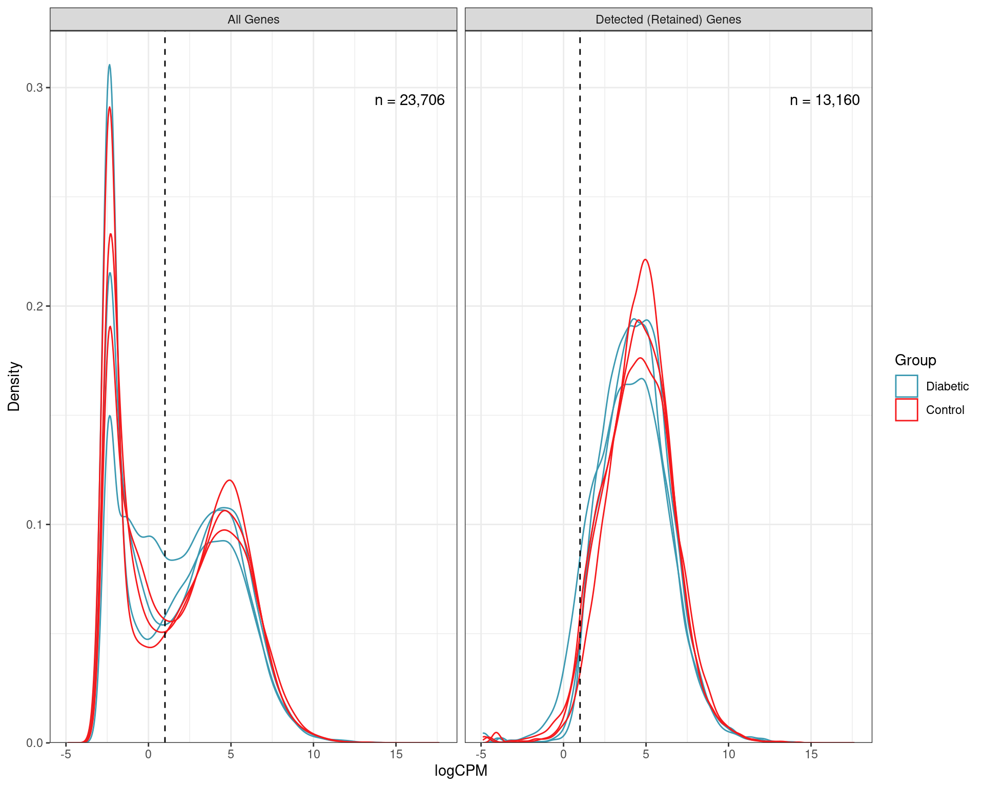
Distributions of logCPM values for all non-zero genes, and those retained as detected using the above CPM threshold. The number of genes in each category is also shown.
| Version | Author | Date |
|---|---|---|
| fcfd11c | Steve Pederson | 2022-07-07 |
RLE
voomData$E %>%
  as.data.frame() %>%
  pivot_longer(
    cols = everything(), names_to = "Rat", values_to = "logCPM"
  ) %>%
  left_join(samples) %>%
  group_by(Rat) %>%
  mutate(RLE = logCPM - median(logCPM))%>%
  ggplot(aes(Rat, RLE, fill = group)) +
  geom_boxplot(alpha = 0.9) +
  geom_hline(yintercept = 0, linetype = 2) +
  facet_wrap(~group, scales = "free_x") +
  scale_fill_manual(values = group_cols) +
  labs(
    x = "Sample", fill = "Group"
  )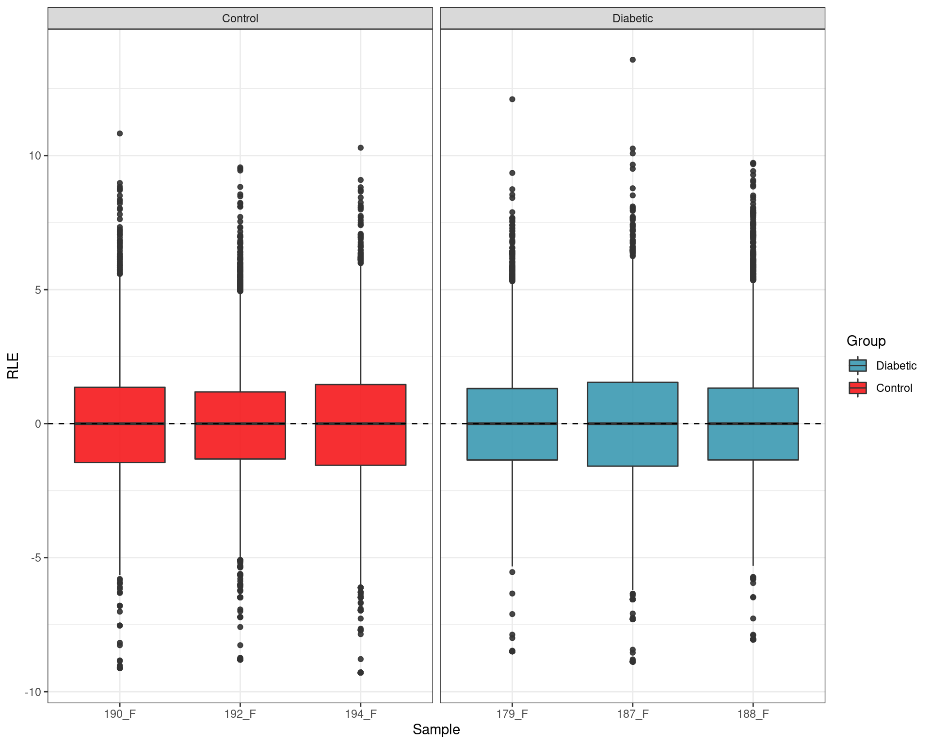
Relative Log Expression. Any deviations from zero indicate potential batch effects, with none being evident.
| Version | Author | Date |
|---|---|---|
| fcfd11c | Steve Pederson | 2022-07-07 |
PCA
pcaPost <- voomData$E %>%
  .[rowVars(.) > 0,] %>%
  t() %>%
  prcomp()
pcaPost %>%
  tidy() %>%
  dplyr::rename(Rat = row) %>%
  left_join(voomData$targets, by = "Rat") %>%
  dplyr::filter(PC %in% 1:2) %>%
  pivot_wider(names_from = "PC", names_prefix = "PC", values_from = "value") %>%
  ggplot(
    aes(PC1, PC2, colour = group, size = lib.size/1e6)
  ) +
  geom_point() +
  geom_text_repel(aes(label = Rat), show.legend = FALSE) +
  scale_colour_manual(values = group_cols) +
  scale_size_continuous(limits = c(5, 15), breaks = seq(5, 15, by = 5)) +
  labs(
    x = glue("PC1 ({percent(pcaPost$sdev[[1]]^2 / sum(pcaPost$sdev^2), 0.1)})"),
    y = glue("PC2 ({percent(pcaPost$sdev[[2]]^2 / sum(pcaPost$sdev^2), 0.1)})"),
    colour = "Group",
    size = "Library Size\n(millions)"
  )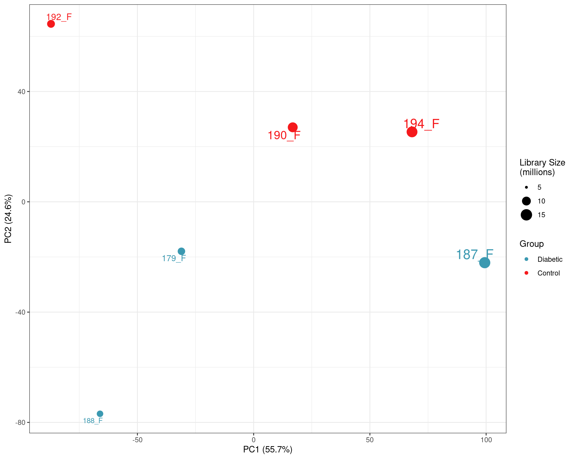
PCA on logCPM values. The clear impact of the smaller libraries is seen with library size being the lragest source of variability. This supports the previous caution that the libraries below 10m reads are not as representative of the true RNA content of the source material. The small final library size after assigning reads to genes also highlights the poor performance of total RNA in this context, given that all raw sequencing libraries were >35 million reads.
| Version | Author | Date |
|---|---|---|
| fcfd11c | Steve Pederson | 2022-07-07 |
Sample Weights
voomData$targets %>%
  ggplot(aes(Rat, sample.weights, fill = group)) +
  geom_col() +
  facet_wrap(~group, scales = "free_x") +
  scale_fill_manual(values = group_cols)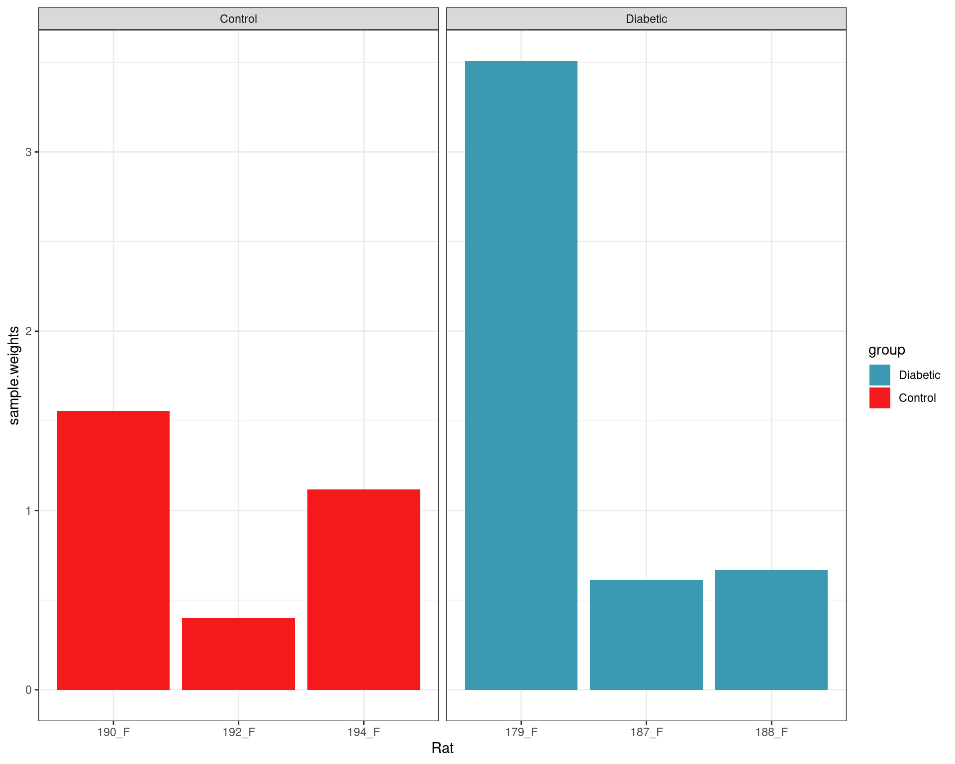
Sample weights after fitting the voom model.
| Version | Author | Date |
|---|---|---|
| fcfd11c | Steve Pederson | 2022-07-07 |
Results
Or the genes retained as confidently detected, 7 were formally considered as DE, using an FDR of 0.05. These were Pnpla2, LOC100909761, Rcor2, Cxcl1, Mmp3, Mmp10 and Il6.
htmltools::tags$caption(
  htmltools::em(
    glue(
      "
      All {sum(results$FDR < 0.1)} genes with an FDR < 0.1 for differential
      expression. Of these, only {sum(results$FDR < 0.05)} made the more formal
      criteria of an FDR < 0.05 for significant differential expression, as
      indicated by the final column. Values in the logFC column represent the
      estimated change in expression on the log2 scale. The AveExpr column
      indicates the average expression level, with the most highly expressed
      gene in the dataset receiving a value of {round(max(results$AveExpr), 2)}.
      The lowest expressed gene which passed the criteria for detection received
      a value of {round(min(results$AveExpr), 2)}, marking this as the effective
      lower limit of detection.
      "
    )
  )
)fs <- 12
results %>%
dplyr::filter(FDR < 0.1) %>%
reactable(
pagination = FALSE,
columns = list(
gene_id = colDef(name = "Gene ID", minWidth = 160),
gene_name = colDef(
name = "Gene",
style = list(fontStyle = "italic")
),
logFC = colDef(
format = colFormat(digits = 2),
style = function(value) {
col <- ifelse(value > 0, "green", "red")
list(color = col)
},
maxWidth = 100
),
AveExpr = colDef(
format = colFormat(digits = 2),
maxWidth = 100
),
t = colDef(format = colFormat(digits = 2), maxWidth = 100),
P.Value = colDef(
name = "p",
cell = function(value) {
fmt <- ifelse(value < 0.01, "%.2e", "%.3f")
sprintf(fmt, value)
},
maxWidth = 120
),
FDR = colDef(
cell = function(value) {
fmt <- ifelse(value < 0.01, "%.2e", "%.3f")
sprintf(fmt, value)
},
maxWidth = 120
),
DE = colDef(
html = TRUE,
cell = function(value) ifelse(value, "✔", "\u274c"),
style = function(value) {
col <- ifelse(value, "green", "red")
list(color = col)
},
maxWidth = 80
)
),
theme = reactableTheme(style = list(fontSize = fs))
)MA Plot
results %>%
  ggplot(aes(AveExpr, logFC)) +
  geom_point(aes(colour = DE),alpha = 0.5) +
  geom_text_repel(
    aes(label = gene_name, colour = DE),
    data = . %>%
      arrange(desc(abs(logFC))) %>%
      dplyr::filter(FDR < 0.1),
    show.legend = FALSE
  ) +
  geom_smooth(se = FALSE) +
  scale_colour_manual(values = c("grey50", "red")) +
  theme(legend.position = "none")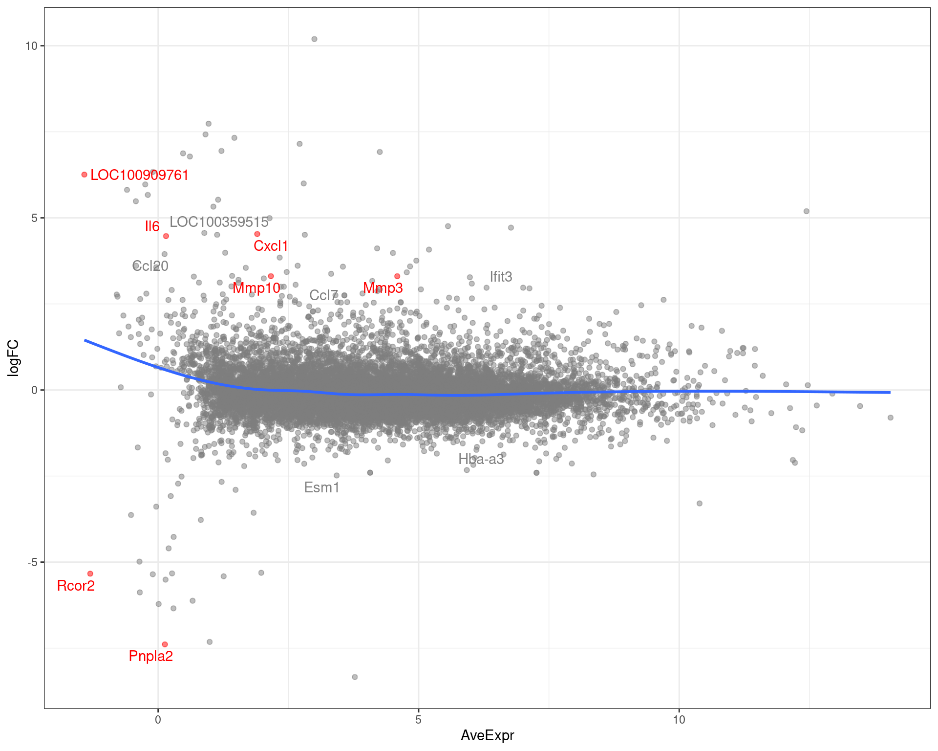
MA-plot showing all genes with an FDR < 0.1. Those passing the FDR threshold of 0.05 are highlighted in red.
| Version | Author | Date |
|---|---|---|
| fcfd11c | Steve Pederson | 2022-07-07 |
Volcano Plot
results %>%
  ggplot(aes(logFC, -log10(P.Value))) +
  geom_point(aes(colour = DE),alpha = 0.5) +
  geom_text_repel(
    aes(label = gene_name, colour = DE),
    data = . %>%
      arrange(desc(abs(logFC))) %>%
      dplyr::filter(FDR < 0.1),
    show.legend = FALSE
  ) +
  scale_colour_manual(values = c("grey50", "red")) +
  theme(legend.position = "none") +
  labs(y = expression(paste(-log[10], "p")))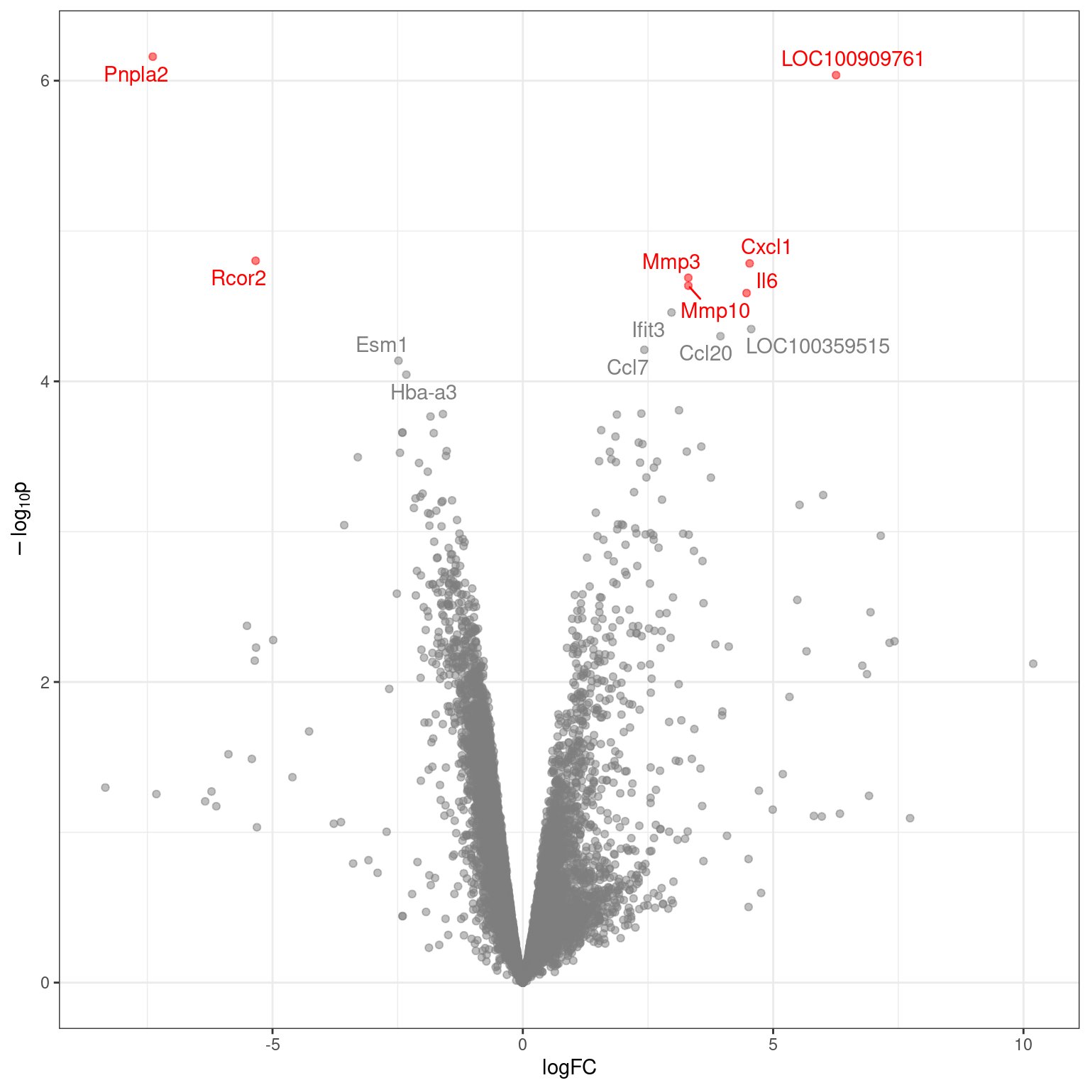
Volcano plot with genes labelled to an FDR of 0.1. DE genes to an FDR threshold of 0.05 are highlighted in red.
| Version | Author | Date |
|---|---|---|
| fcfd11c | Steve Pederson | 2022-07-07 |
Highly Ranked Genes
results %>%
  dplyr::slice(1:12) %>%
  mutate(
    gene_name = case_when(
      DE ~ paste0(gene_name, "*"),
      TRUE ~ gene_name
    )
  ) %>%
  dplyr::select(gene_id, gene_name) %>%
  bind_cols(
    voomData[.$gene_id,]$E
  ) %>%
  pivot_longer(
    cols = all_of(samples$Rat),
    names_to = "Rat", values_to = "logCPM"
  ) %>%
  left_join(
    dplyr::select(voomData$targets, Rat, group, sample.weights)
  ) %>%
  mutate(gene_name = fct_inorder(gene_name)) %>%
  ggplot(
    aes(group, logCPM, fill = group)
  ) +
  geom_boxplot() +
  geom_hline(yintercept = log2(min_cpm), linetype = 2, colour = "grey30") +
  facet_wrap(~gene_name) +
  labs(x = "Group", fill = "Group")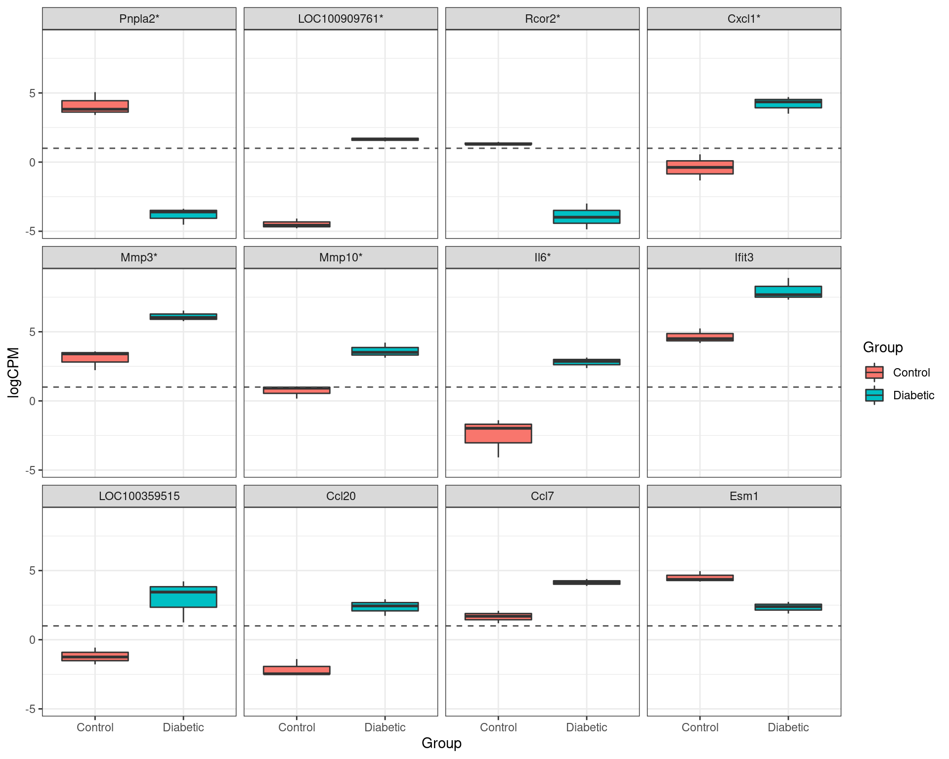
The most highly ranked genes for differential expression. Those formally passing the criteria for differential expression (FDR < 0.05) are marked with an asterisk.
| Version | Author | Date |
|---|---|---|
| fcfd11c | Steve Pederson | 2022-07-07 |
write_csv(results, here::here("output/top_table.csv"))Enrichment Analysis
rankedGenes <- results %>%
  arrange(t) %>%
  with(
    structure(t, names = gene_id)
  )
msigdb <- msigdbr(species = "Rattus norvegicus") %>%
  dplyr::filter(
    gs_cat %in% c("H", "C5") |
      gs_subcat %in% c("CP:KEGG", "CP:REACTOME", "CP:WIKIPATHWAYS", "IMMUNESIGDB")
  ) %>%
  dplyr::filter(ensembl_gene %in% names(rankedGenes))
gsByPathway <- msigdb %>%
  split(.$gs_name) %>%
  lapply(pull, "ensembl_gene") %>%
  .[vapply(., length, integer(1)) > 5]
id2Name <- structure(
  genesGR$gene_name,
  names = genesGR$gene_id
) %>%
  .[!duplicated(names(.))]
Given the low number of differentially expressed genes, GSEA was used
as implemented in the R package fgsea, with the ranked list
of genes generated using the t-statistics as obtained above.
Enrichment analysis was performed on gene-sets obtained from MSigDB version 7.5. Gene sets were selected from HALLMARK, KEGG, REACTOME, WIkiPathways, ImmuneSigDB and the Gene Ontology Database. Only the 19,499 gene-sets with more than 5 genes detected in the dataset were retained. P-values obtained from GSEA were adjusted using Bonferroni’s method to ensure strong control of the Family-Wise Error Rate (FWER).
gseaResults <- fgsea(gsByPathway, rankedGenes, BPPARAM = bpparam) %>%
  arrange(pval) %>%
  mutate(padj = p.adjust(pval, "bonf")) %>%
  dplyr::select(gs_name = pathway, pval, padj, NES, size, leadingEdge) %>%
  left_join(
    distinct(msigdb, gs_name, gs_cat, gs_subcat)
  )
HALLMARK Gene Sets
Results
df <- gseaResults %>%
  dplyr::filter(gs_cat == "H", padj < 0.01) %>%
  mutate(
    leSize = vapply(leadingEdge, length, integer(1)),
   leadingEdge = vapply(
     leadingEdge,
     function(x) paste(id2Name[x], collapse = "; "),
     character(1)
   )
  ) %>%
  dplyr::select(gs_name, pval, padj, NES, ends_with("size"), leadingEdge)
htmltools::tags$caption(
  htmltools::em(
    glue(
      "
      All {nrow(df)} HALLMARK gene sets considered to be enriched in the ranked
      list of genes. All p-values are Bonferroni-adjusted with p < 0.01 used for
      significance. A Normalised Enrichment Score
      (NES) > 0 indicates that the geneset was enriched amongst
      up-regulated genes, whilst a negative NES indicates enrichment in the
      down-regulated genes. Genes in the Leading Edge represent those which
      appear in the ranked list up until the point of the most extreme NES.
      "
    )
  )
)df %>%
reactable(
searchable = TRUE, filterable = TRUE,
columns = list(
gs_name = colDef(
name = "Gene Set",
cell = function(value) str_replace_all(value, "_", " ")
),
pval = colDef(show = FALSE),
padj = colDef(
name = "p<sub>adj</sub>", html = TRUE,
cell = function(value) {
fmt <- "%.2e"
if (value > 0.001) fmt <- "%.3f"
sprintf(fmt, value)
},
maxWidth = 100
),
NES = colDef(
format = colFormat(digits = 2),
maxWidth = 80
),
size = colDef(name = "Gene Set Size", maxWidth = 100),
leSize = colDef(name = "Leading Edge Size", maxWidth = 100),
leadingEdge = colDef(
name = "Leading Edge",
cell = function(value) with_tooltip(value, width = 50)
)
)
)Plots
p <- df %>%
  dplyr::slice(1:9) %>%
  pull("gs_name") %>%
  lapply(
    function(x) {
      plotEnrichment(gsByPathway[[x]], rankedGenes) +
        ggtitle(
          str_replace_all(x, "_", " ") %>%
            str_trunc(40)
        ) +
        ylim(0.62 * c(-1, 1)) +
        theme(plot.title = element_text(hjust = 0.5, size = 10))
    }
  )
plot_grid(plotlist = p)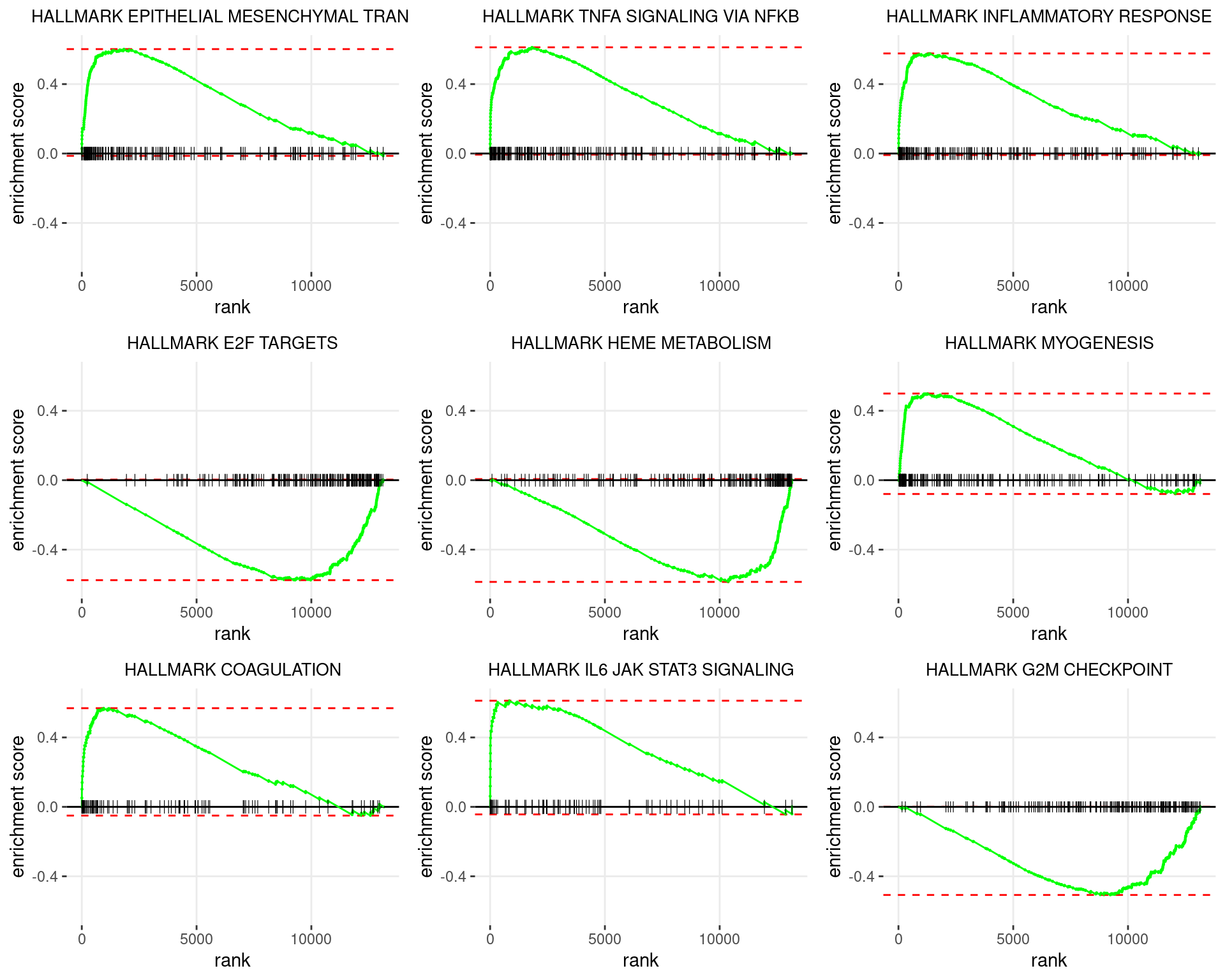
Enrichment plots for the most highly ranked HALLMARK gene-sets, showing the approximate position within the ranked list where the maximal enrichment score is found. The most compelling results will always be associated with maximal enrichment scores near either extreme.
| Version | Author | Date |
|---|---|---|
| fcfd11c | Steve Pederson | 2022-07-07 |
df %>%
  write_csv(
    here::here("output/hallmark_gsea.csv")
  )
Reactome Gene Sets
Results
df <- gseaResults %>%
  dplyr::filter(gs_subcat == "CP:REACTOME", padj < 0.05) %>%
  mutate(
    leSize = vapply(leadingEdge, length, integer(1)),
   leadingEdge = vapply(
     leadingEdge,
     function(x) paste(id2Name[x], collapse = "; "),
     character(1)
   )
  ) %>%
  dplyr::select(gs_name, pval, padj, NES, ends_with("size"), leadingEdge)
htmltools::tags$caption(
  htmltools::em(
    glue(
      "
      All {nrow(df)} Reactome gene sets considered to be enriched in the ranked
      list of genes.
      All p-values are Bonferroni-adjusted. A Normalised Enrichment Score
      (NES) > 0 indicates that the geneset was enriched amongst
      up-regulated genes, whilst a negative NES indicates enrichment in the
      down-regulated genes. Genes in the Leading Edge represent those which
      appear in the ranked list up until the point of the most extreme NES.
      "
    )
  )
)df %>%
reactable(
searchable = TRUE, filterable = TRUE,
columns = list(
gs_name = colDef(
name = "Gene Set",
cell = function(value) str_replace_all(value, "_", " ")
),
pval = colDef(show = FALSE),
padj = colDef(
name = "p<sub>adj</sub>", html = TRUE,
cell = function(value) {
fmt <- "%.2e"
if (value > 0.001) fmt <- "%.3f"
sprintf(fmt, value)
},
maxWidth = 100
),
NES = colDef(
format = colFormat(digits = 2),
maxWidth = 80
),
size = colDef(name = "Gene Set Size", maxWidth = 100),
leSize = colDef(name = "Leading Edge Size", maxWidth = 100),
leadingEdge = colDef(
name = "Leading Edge",
cell = function(value) with_tooltip(value, width = 50)
)
)
)Plots
p <- df %>%
  dplyr::slice(1:9) %>%
  pull("gs_name") %>%
  lapply(
    function(x) {
      plotEnrichment(gsByPathway[[x]], rankedGenes) +
        ggtitle(
          str_replace_all(x, "_", " ") %>%
            str_trunc(40)
        ) +
        ylim(0.6 * c(-1, 1)) +
        theme(plot.title = element_text(hjust = 0.5, size = 10))
    }
  )
plot_grid(plotlist = p)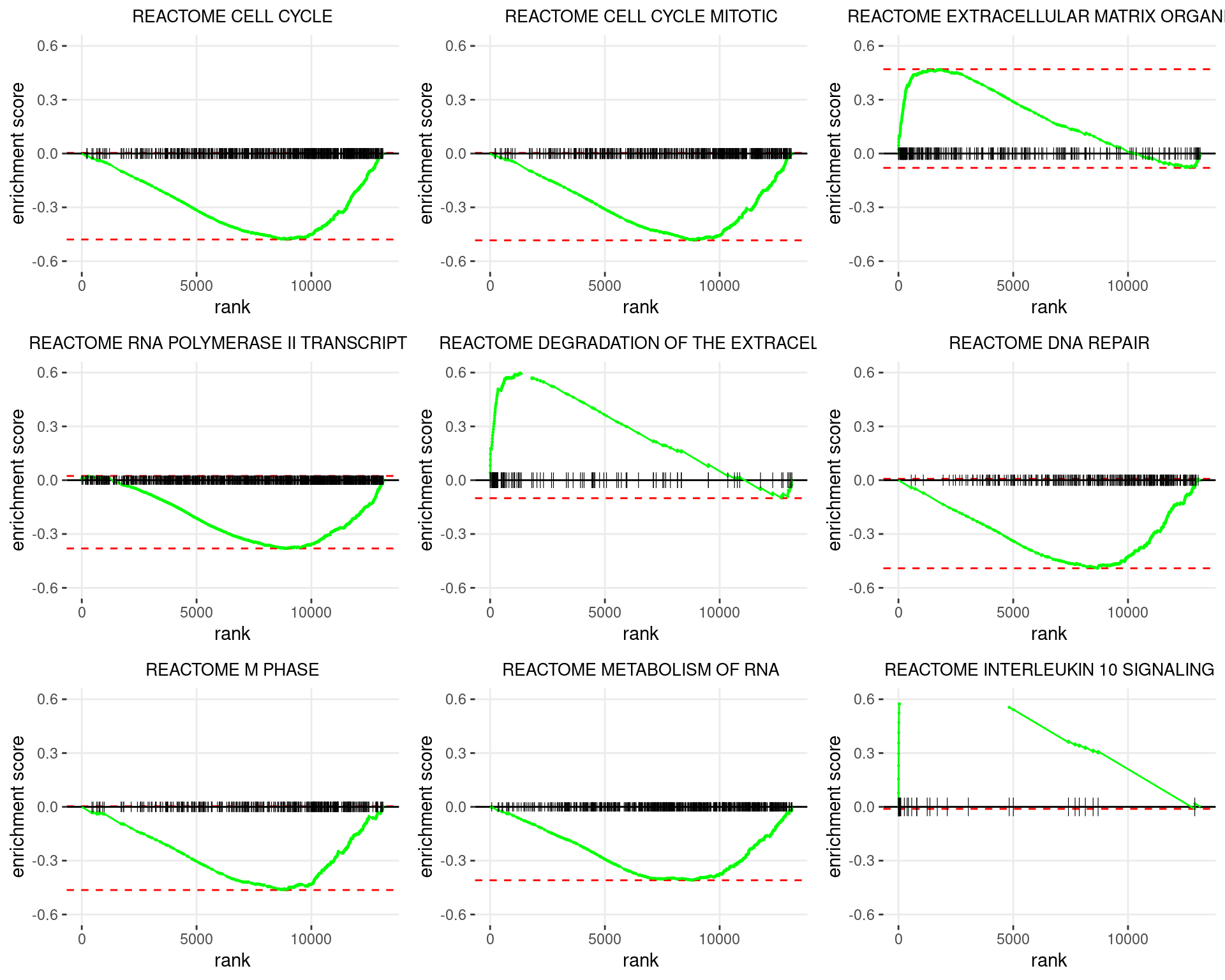
Enrichment plots for the most highly ranked Reactome gene-sets, showing the approximate position within the ranked list where the maximal enrichment score is found. The most compelling results will always be associated with maximal enrichment scores near either extreme.
| Version | Author | Date |
|---|---|---|
| fcfd11c | Steve Pederson | 2022-07-07 |
KEGG Gene Sets
Results
df <- gseaResults %>%
  dplyr::filter(gs_subcat == "CP:KEGG", padj < 0.05) %>%
  mutate(
    leSize = vapply(leadingEdge, length, integer(1)),
   leadingEdge = vapply(
     leadingEdge,
     function(x) paste(id2Name[x], collapse = "; "),
     character(1)
   )
  ) %>%
  dplyr::select(gs_name, pval, padj, NES, ends_with("size"), leadingEdge)
htmltools::tags$caption(
  htmltools::em(
    glue(
      "
      All {nrow(df)} KEGG gene sets considered to be enriched in the ranked
      list of genes.
      All p-values are Bonferroni-adjusted. A Normalised Enrichment Score
      (NES) > 0 indicates that the geneset was enriched amongst
      up-regulated genes, whilst a negative NES indicates enrichment in the
      down-regulated genes. Genes in the Leading Edge represent those which
      appear in the ranked list up until the point of the most extreme NES.
      "
    )
  )
)df %>%
reactable(
searchable = TRUE, filterable = TRUE,
columns = list(
gs_name = colDef(
name = "Gene Set",
cell = function(value) str_replace_all(value, "_", " ")
),
pval = colDef(show = FALSE),
padj = colDef(
name = "p<sub>adj</sub>", html = TRUE,
cell = function(value) {
fmt <- "%.2e"
if (value > 0.001) fmt <- "%.3f"
sprintf(fmt, value)
},
maxWidth = 100
),
NES = colDef(
format = colFormat(digits = 2),
maxWidth = 80
),
size = colDef(name = "Gene Set Size", maxWidth = 100),
leSize = colDef(name = "Leading Edge Size", maxWidth = 100),
leadingEdge = colDef(
name = "Leading Edge",
cell = function(value) with_tooltip(value, width = 50)
)
)
)Plots
p <- df %>%
  dplyr::slice(1:9) %>%
  pull("gs_name") %>%
  lapply(
    function(x) {
      plotEnrichment(gsByPathway[[x]], rankedGenes) +
        ggtitle(
          str_replace_all(x, "_", " ") %>%
            str_trunc(40)
        ) +
        ylim(0.62 * c(-1, 1)) +
        theme(plot.title = element_text(hjust = 0.5, size = 10))
    }
  )
plot_grid(plotlist = p)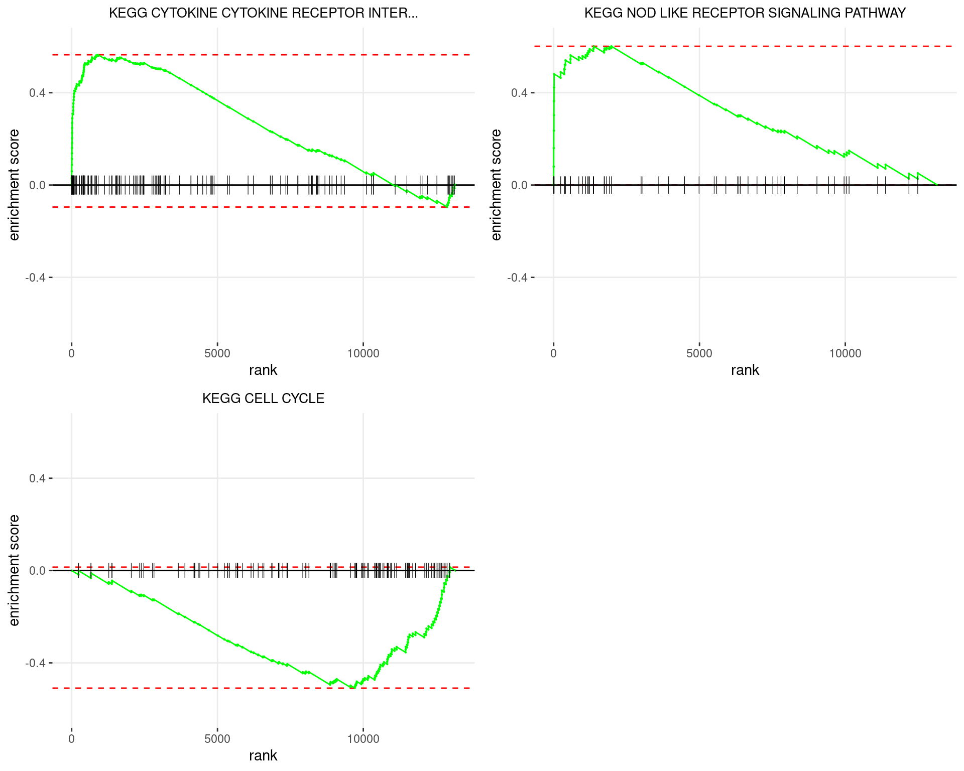
Enrichment plots for the most highly ranked KEGG gene-sets, showing the approximate position within the ranked list where the maximal enrichment score is found. The most compelling results will always be associated with maximal enrichment scores near either extreme.
| Version | Author | Date |
|---|---|---|
| fcfd11c | Steve Pederson | 2022-07-07 |
WIKIPATHWAYS Gene Sets
Results
df <- gseaResults %>%
  dplyr::filter(gs_subcat == "CP:WIKIPATHWAYS", padj < 0.05) %>%
  mutate(
    leSize = vapply(leadingEdge, length, integer(1)),
   leadingEdge = vapply(
     leadingEdge,
     function(x) paste(id2Name[x], collapse = "; "),
     character(1)
   )
  ) %>%
  dplyr::select(gs_name, pval, padj, NES, ends_with("size"), leadingEdge)
htmltools::tags$caption(
  htmltools::em(
    glue(
      "
      All {nrow(df)} WIKIPATHWAYS gene sets considered to be enriched in the
      ranked list of genes.
      All p-values are Bonferroni-adjusted. A Normalised Enrichment Score
      (NES) > 0 indicates that the geneset was enriched amongst
      up-regulated genes, whilst a negative NES indicates enrichment in the
      down-regulated genes. Genes in the Leading Edge represent those which
      appear in the ranked list up until the point of the most extreme NES.
      "
    )
  )
)df %>%
reactable(
searchable = TRUE, filterable = TRUE,
columns = list(
gs_name = colDef(
name = "Gene Set",
cell = function(value) str_replace_all(value, "_", " ")
),
pval = colDef(show = FALSE),
padj = colDef(
name = "p<sub>adj</sub>", html = TRUE,
cell = function(value) {
fmt <- "%.2e"
if (value > 0.001) fmt <- "%.3f"
sprintf(fmt, value)
},
maxWidth = 100
),
NES = colDef(
format = colFormat(digits = 2),
maxWidth = 80
),
size = colDef(name = "Gene Set Size", maxWidth = 100),
leSize = colDef(name = "Leading Edge Size", maxWidth = 100),
leadingEdge = colDef(
name = "Leading Edge",
cell = function(value) with_tooltip(value, width = 50)
)
)
)Plots
p <- df %>%
  dplyr::slice(1:9) %>%
  pull("gs_name") %>%
  lapply(
    function(x) {
      plotEnrichment(gsByPathway[[x]], rankedGenes) +
        ggtitle(
          str_replace_all(x, "_", " ") %>%
            str_trunc(40)
        ) +
        ylim(0.9 * c(-1, 1)) +
        theme(plot.title = element_text(hjust = 0.5, size = 10))
    }
  )
plot_grid(plotlist = p)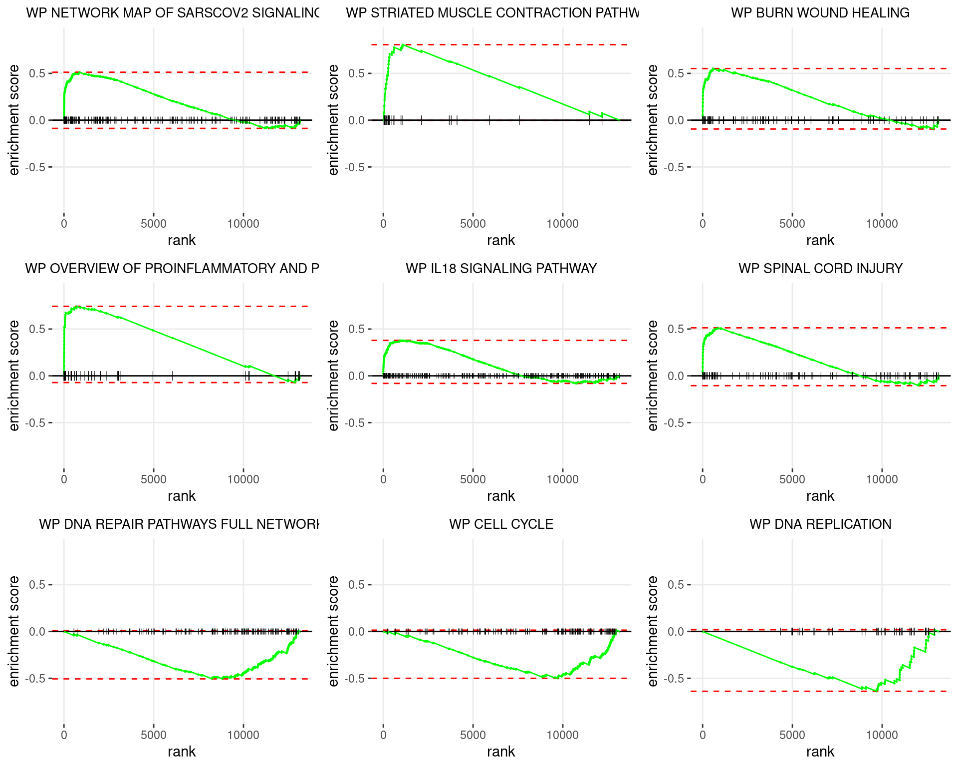
Enrichment plots for the most highly ranked WIKIPATHWAYS gene-sets, showing the approximate position within the ranked list where the maximal enrichment score is found. The most compelling results will always be associated with maximal enrichment scores near either extreme.
| Version | Author | Date |
|---|---|---|
| fcfd11c | Steve Pederson | 2022-07-07 |
ImmunSigDB Gene Sets
Results
df <- gseaResults %>%
  dplyr::filter(gs_subcat == "IMMUNESIGDB", padj < 0.05) %>%
  mutate(
    leSize = vapply(leadingEdge, length, integer(1)),
   leadingEdge = vapply(
     leadingEdge,
     function(x) paste(id2Name[x], collapse = "; "),
     character(1)
   )
  ) %>%
  dplyr::select(gs_name, pval, padj, NES, ends_with("size"), leadingEdge)
htmltools::tags$caption(
  htmltools::em(
    glue(
      "
      All {nrow(df)} ImmunSigDB gene sets considered to be enriched in the
      ranked list of genes.
      All p-values are Bonferroni-adjusted. A Normalised Enrichment Score
      (NES) > 0 indicates that the geneset was enriched amongst
      up-regulated genes, whilst a negative NES indicates enrichment in the
      down-regulated genes. Genes in the Leading Edge represent those which
      appear in the ranked list up until the point of the most extreme NES.
      "
    )
  )
)df %>%
reactable(
searchable = TRUE, filterable = TRUE,
columns = list(
gs_name = colDef(
name = "Gene Set",
cell = function(value) str_replace_all(value, "_", " ")
),
pval = colDef(show = FALSE),
padj = colDef(
name = "p<sub>adj</sub>", html = TRUE,
cell = function(value) {
fmt <- "%.2e"
if (value > 0.001) fmt <- "%.3f"
sprintf(fmt, value)
},
maxWidth = 100
),
NES = colDef(
format = colFormat(digits = 2),
maxWidth = 80
),
size = colDef(name = "Gene Set Size", maxWidth = 100),
leSize = colDef(name = "Leading Edge Size", maxWidth = 100),
leadingEdge = colDef(
name = "Leading Edge",
cell = function(value) with_tooltip(value, width = 50)
)
)
)Plots
p <- df %>%
  dplyr::slice(1:9) %>%
  pull("gs_name") %>%
  lapply(
    function(x) {
      plotEnrichment(gsByPathway[[x]], rankedGenes) +
        ggtitle(
          str_replace_all(x, "_", " ") %>%
            str_trunc(40)
        ) +
        ylim(0.6 * c(-1, 1)) +
        theme(plot.title = element_text(hjust = 0.5, size = 10))
    }
  )
plot_grid(plotlist = p)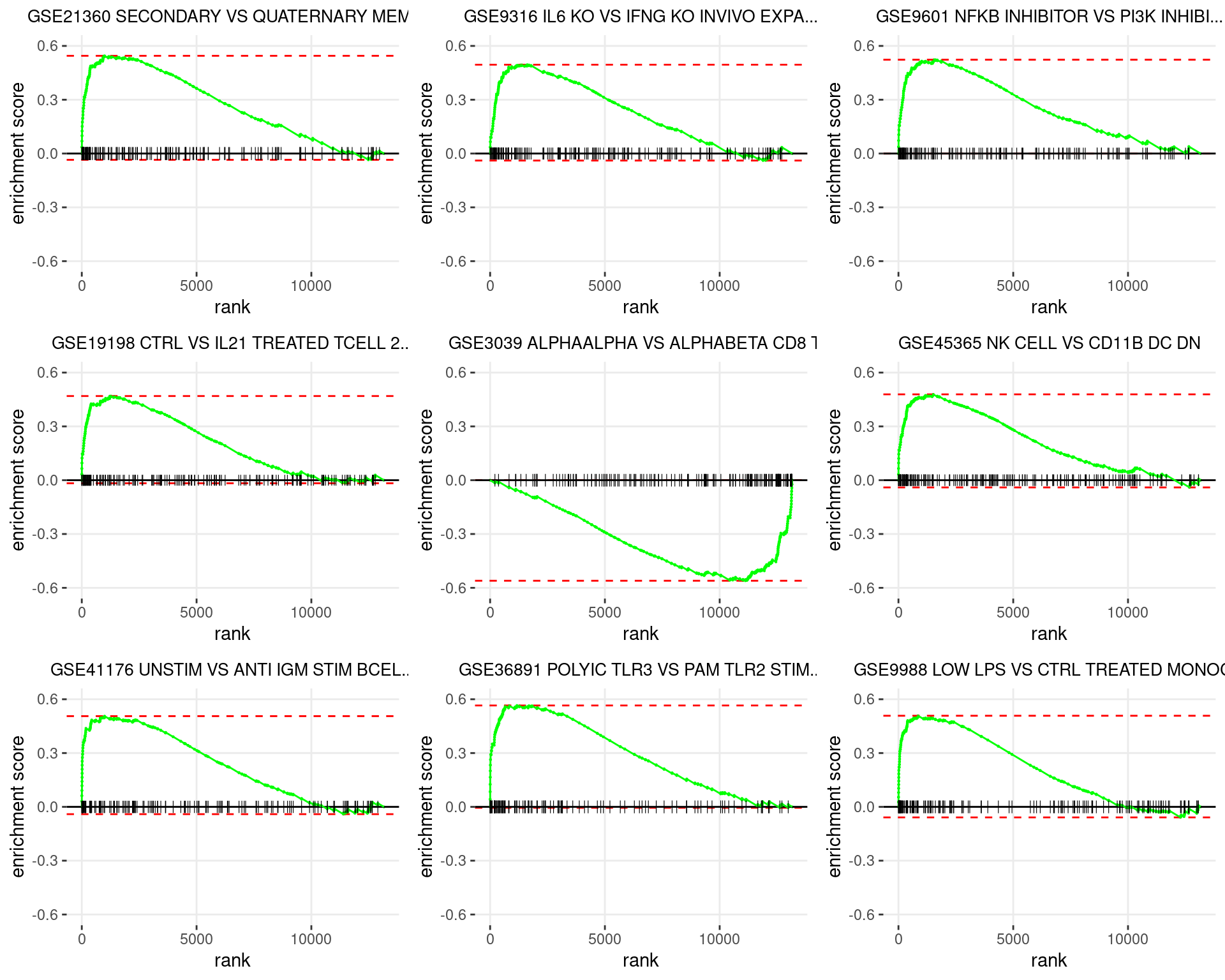
Enrichment plots for the most highly ranked ImmuneSigDB gene-sets, showing the approximate position within the ranked list where the maximal enrichment score is found. The most compelling results will always be associated with maximal enrichment scores near either extreme.
| Version | Author | Date |
|---|---|---|
| fcfd11c | Steve Pederson | 2022-07-07 |
GO: Biological Process Gene Sets
Results
df <- gseaResults %>%
  dplyr::filter(gs_subcat == "GO:BP", padj < 0.05) %>%
  mutate(
    leSize = vapply(leadingEdge, length, integer(1)),
   leadingEdge = vapply(
     leadingEdge,
     function(x) paste(id2Name[x], collapse = "; "),
     character(1)
   )
  ) %>%
  dplyr::select(gs_name, pval, padj, NES, ends_with("size"), leadingEdge)
htmltools::tags$caption(
  htmltools::em(
    glue(
      "
      All {nrow(df)} GO: Biological Process gene sets considered to be enriched
      in the ranked list of genes.
      All p-values are Bonferroni-adjusted. A Normalised Enrichment Score
      (NES) > 0 indicates that the geneset was enriched amongst
      up-regulated genes, whilst a negative NES indicates enrichment in the
      down-regulated genes. Genes in the Leading Edge represent those which
      appear in the ranked list up until the point of the most extreme NES.
      "
    )
  )
)df %>%
reactable(
searchable = TRUE, filterable = TRUE,
columns = list(
gs_name = colDef(
name = "Gene Set",
cell = function(value) str_replace_all(value, "_", " ") %>%
str_remove("^GO(BP|CC|MF) ")
),
pval = colDef(show = FALSE),
padj = colDef(
name = "p<sub>adj</sub>", html = TRUE,
cell = function(value) {
fmt <- "%.2e"
if (value > 0.001) fmt <- "%.3f"
sprintf(fmt, value)
},
maxWidth = 100
),
NES = colDef(
format = colFormat(digits = 2),
maxWidth = 80
),
size = colDef(name = "Gene Set Size", maxWidth = 100),
leSize = colDef(name = "Leading Edge Size", maxWidth = 100),
leadingEdge = colDef(
name = "Leading Edge",
cell = function(value) with_tooltip(value, width = 50)
)
)
)Plots
p <- df %>%
  dplyr::slice(1:9) %>%
  pull("gs_name") %>%
  lapply(
    function(x) {
      plotEnrichment(gsByPathway[[x]], rankedGenes) +
        ggtitle(
          str_replace_all(x, "_", " ") %>%
            str_remove("^GO(BP|CC|MF) ") %>%
            str_trunc(40)
        ) +
        ylim(0.55 * c(-1, 1)) +
        theme(plot.title = element_text(hjust = 0.5, size = 10))
    }
  )
plot_grid(plotlist = p)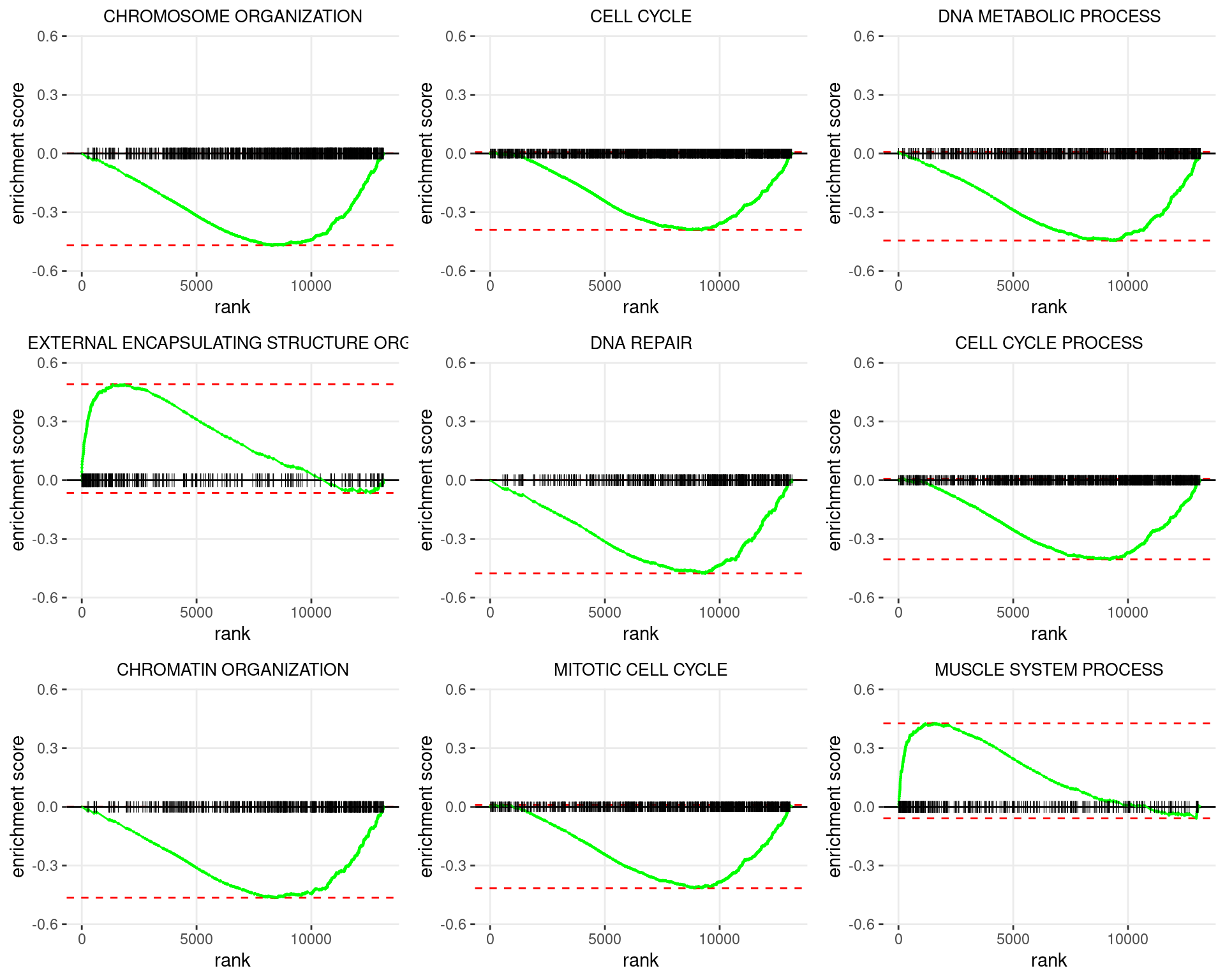
Enrichment plots for the most highly ranked GO: Biological Process gene-sets, showing the approximate position within the ranked list where the maximal enrichment score is found. The most compelling results will always be associated with maximal enrichment scores near either extreme.
| Version | Author | Date |
|---|---|---|
| fcfd11c | Steve Pederson | 2022-07-07 |
GO: Cellular Component Gene Sets
Results
df <- gseaResults %>%
  dplyr::filter(gs_subcat == "GO:MF", padj < 0.05) %>%
  mutate(
    leSize = vapply(leadingEdge, length, integer(1)),
   leadingEdge = vapply(
     leadingEdge,
     function(x) paste(id2Name[x], collapse = "; "),
     character(1)
   )
  ) %>%
  dplyr::select(gs_name, pval, padj, NES, ends_with("size"), leadingEdge)
htmltools::tags$caption(
  htmltools::em(
    glue(
      "
      All {nrow(df)} GO: Molecular Function gene sets considered to be enriched
      in the ranked list of genes.
      All p-values are Bonferroni-adjusted. A Normalised Enrichment Score
      (NES) > 0 indicates that the geneset was enriched amongst
      up-regulated genes, whilst a negative NES indicates enrichment in the
      down-regulated genes. Genes in the Leading Edge represent those which
      appear in the ranked list up until the point of the most extreme NES.
      "
    )
  )
)df %>%
reactable(
searchable = TRUE, filterable = TRUE,
columns = list(
gs_name = colDef(
name = "Gene Set",
cell = function(value) str_replace_all(value, "_", " ") %>%
str_remove("^GO(BP|CC|MF) ")
),
pval = colDef(show = FALSE),
padj = colDef(
name = "p<sub>adj</sub>", html = TRUE,
cell = function(value) {
fmt <- "%.2e"
if (value > 0.001) fmt <- "%.3f"
sprintf(fmt, value)
},
maxWidth = 100
),
NES = colDef(
format = colFormat(digits = 2),
maxWidth = 80
),
size = colDef(name = "Gene Set Size", maxWidth = 100),
leSize = colDef(name = "Leading Edge Size", maxWidth = 100),
leadingEdge = colDef(
name = "Leading Edge",
cell = function(value) with_tooltip(value, width = 50)
)
)
)Plots
p <- df %>%
  dplyr::slice(1:9) %>%
  pull("gs_name") %>%
  lapply(
    function(x) {
      plotEnrichment(gsByPathway[[x]], rankedGenes) +
        ggtitle(
          str_replace_all(x, "_", " ") %>%
            str_remove("^GO(BP|CC|MF) ") %>%
            str_trunc(40)
        ) +
        ylim(0.7 * c(-1, 1)) +
        theme(plot.title = element_text(hjust = 0.5, size = 10))
    }
  )
plot_grid(plotlist = p)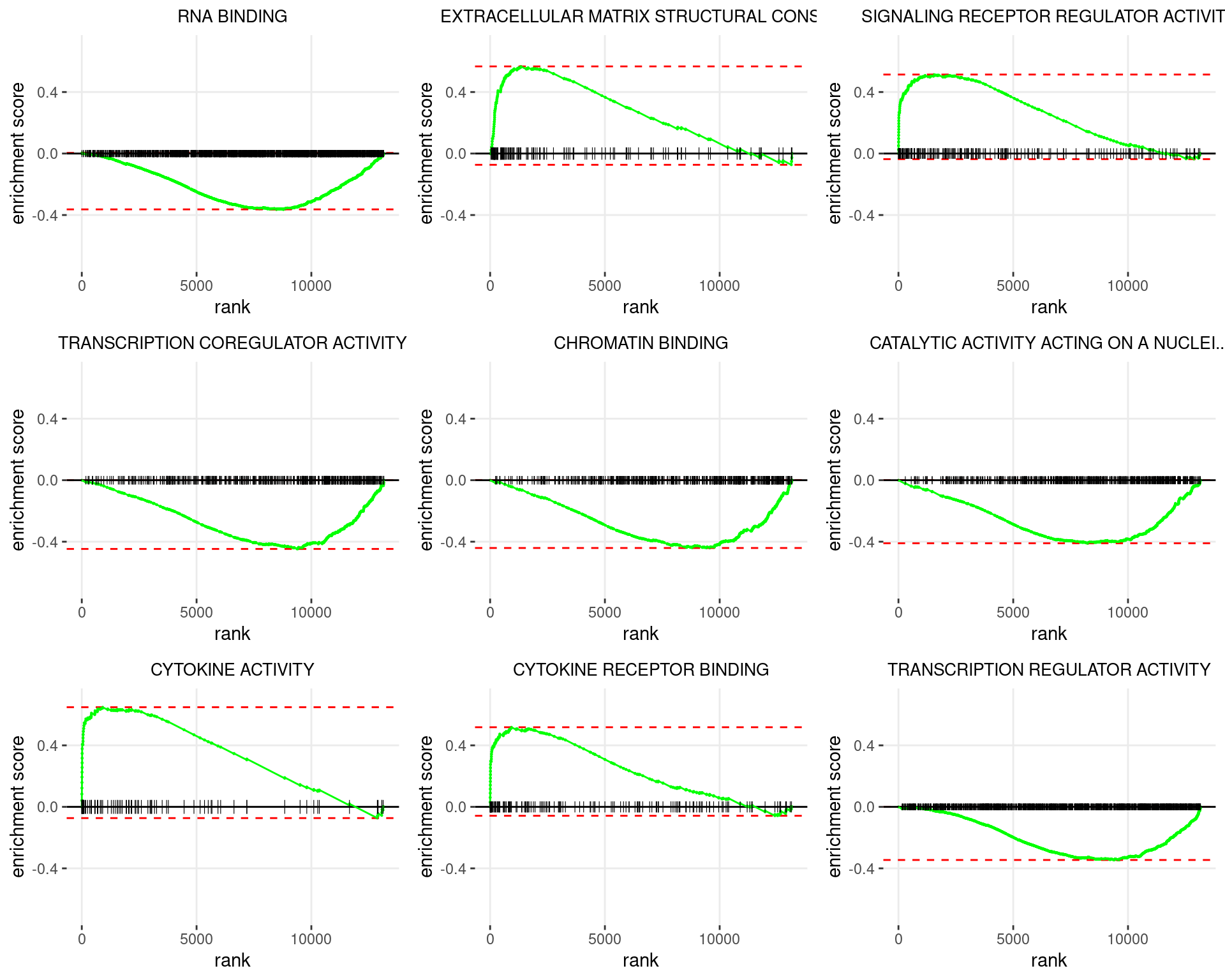
Enrichment plots for the most highly ranked GO: Molecular Function gene-sets, showing the approximate position within the ranked list where the maximal enrichment score is found. The most compelling results will always be associated with maximal enrichment scores near either extreme.
| Version | Author | Date |
|---|---|---|
| fcfd11c | Steve Pederson | 2022-07-07 |
GO: Molecular Function Gene Sets
Results
df <- gseaResults %>%
  dplyr::filter(gs_subcat == "GO:CC", padj < 0.05) %>%
  mutate(
    leSize = vapply(leadingEdge, length, integer(1)),
   leadingEdge = vapply(
     leadingEdge,
     function(x) paste(id2Name[x], collapse = "; "),
     character(1)
   )
  ) %>%
  dplyr::select(gs_name, pval, padj, NES, ends_with("size"), leadingEdge)
htmltools::tags$caption(
  htmltools::em(
    glue(
      "
      All {nrow(df)} GO: Cellular Component gene sets considered to be enriched
      in the ranked list of genes.
      All p-values are Bonferroni-adjusted. A Normalised Enrichment Score
      (NES) > 0 indicates that the geneset was enriched amongst
      up-regulated genes, whilst a negative NES indicates enrichment in the
      down-regulated genes. Genes in the Leading Edge represent those which
      appear in the ranked list up until the point of the most extreme NES.
      "
    )
  )
)df %>%
reactable(
searchable = TRUE, filterable = TRUE,
columns = list(
gs_name = colDef(
name = "Gene Set",
cell = function(value) str_replace_all(value, "_", " ") %>%
str_remove("^GO(BP|CC|MF) ")
),
pval = colDef(show = FALSE),
padj = colDef(
name = "p<sub>adj</sub>", html = TRUE,
cell = function(value) {
fmt <- "%.2e"
if (value > 0.001) fmt <- "%.3f"
sprintf(fmt, value)
},
maxWidth = 100
),
NES = colDef(
format = colFormat(digits = 2),
maxWidth = 80
),
size = colDef(name = "Gene Set Size", maxWidth = 100),
leSize = colDef(name = "Leading Edge Size", maxWidth = 100),
leadingEdge = colDef(
name = "Leading Edge",
cell = function(value) with_tooltip(value, width = 50)
)
)
)Plots
p <- df %>%
  dplyr::slice(1:9) %>%
  pull("gs_name") %>%
  lapply(
    function(x) {
      plotEnrichment(gsByPathway[[x]], rankedGenes) +
        ggtitle(
          str_replace_all(x, "_", " ") %>%
            str_remove("^GO(BP|CC|MF) ") %>%
            str_trunc(40)
        ) +
        ylim(0.55 * c(-1, 1)) +
        theme(plot.title = element_text(hjust = 0.5, size = 10))
    }
  )
plot_grid(plotlist = p)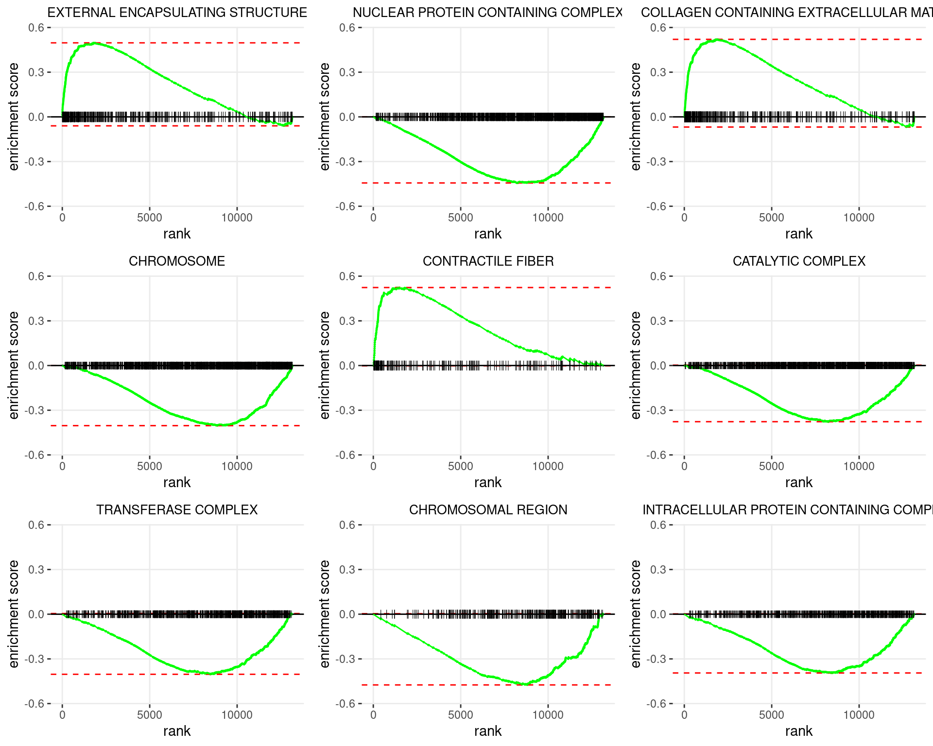
Enrichment plots for the most highly ranked GO: Cellular Component gene-sets, showing the approximate position within the ranked list where the maximal enrichment score is found. The most compelling results will always be associated with maximal enrichment scores near either extreme.
| Version | Author | Date |
|---|---|---|
| fcfd11c | Steve Pederson | 2022-07-07 |
sessionInfo()R version 4.2.0 (2022-04-22)
Platform: x86_64-pc-linux-gnu (64-bit)
Running under: Ubuntu 20.04.4 LTS
Matrix products: default
BLAS: /usr/lib/x86_64-linux-gnu/blas/libblas.so.3.9.0
LAPACK: /usr/lib/x86_64-linux-gnu/lapack/liblapack.so.3.9.0
locale:
[1] LC_CTYPE=en_AU.UTF-8 LC_NUMERIC=C
[3] LC_TIME=en_AU.UTF-8 LC_COLLATE=en_AU.UTF-8
[5] LC_MONETARY=en_AU.UTF-8 LC_MESSAGES=en_AU.UTF-8
[7] LC_PAPER=en_AU.UTF-8 LC_NAME=C
[9] LC_ADDRESS=C LC_TELEPHONE=C
[11] LC_MEASUREMENT=en_AU.UTF-8 LC_IDENTIFICATION=C
attached base packages:
[1] stats4 stats graphics grDevices utils datasets methods
[8] base
other attached packages:
[1] BiocParallel_1.30.0 htmltools_0.5.2 reactable_0.2.3
[4] fgsea_1.22.0 msigdbr_7.5.1 statmod_1.4.36
[7] ggrepel_0.9.1 broom_0.8.0 matrixStats_0.62.0
[10] cowplot_1.1.1 magrittr_2.0.3 ensembldb_2.20.1
[13] AnnotationFilter_1.20.0 GenomicFeatures_1.48.0 AnnotationDbi_1.58.0
[16] Biobase_2.56.0 GenomicRanges_1.48.0 GenomeInfoDb_1.32.1
[19] IRanges_2.30.0 S4Vectors_0.34.0 AnnotationHub_3.4.0
[22] BiocFileCache_2.4.0 dbplyr_2.1.1 BiocGenerics_0.42.0
[25] edgeR_3.38.0 limma_3.52.0 glue_1.6.2
[28] pander_0.6.5 scales_1.2.0 forcats_0.5.1
[31] stringr_1.4.0 dplyr_1.0.9 purrr_0.3.4
[34] readr_2.1.2 tidyr_1.2.0 tibble_3.1.7
[37] ggplot2_3.3.6 tidyverse_1.3.1 workflowr_1.7.0
loaded via a namespace (and not attached):
[1] readxl_1.4.0 backports_1.4.1
[3] fastmatch_1.1-3 lazyeval_0.2.2
[5] splines_4.2.0 crosstalk_1.2.0
[7] digest_0.6.29 fansi_1.0.3
[9] memoise_2.0.1 tzdb_0.3.0
[11] Biostrings_2.64.0 modelr_0.1.8
[13] vroom_1.5.7 prettyunits_1.1.1
[15] colorspace_2.0-3 blob_1.2.3
[17] rvest_1.0.2 rappdirs_0.3.3
[19] haven_2.5.0 xfun_0.30
[21] callr_3.7.0 crayon_1.5.1
[23] RCurl_1.98-1.6 jsonlite_1.8.0
[25] gtable_0.3.0 zlibbioc_1.42.0
[27] XVector_0.36.0 DelayedArray_0.22.0
[29] DBI_1.1.2 Rcpp_1.0.8.3
[31] xtable_1.8-4 progress_1.2.2
[33] bit_4.0.4 htmlwidgets_1.5.4
[35] httr_1.4.3 ellipsis_0.3.2
[37] farver_2.1.0 pkgconfig_2.0.3
[39] XML_3.99-0.9 sass_0.4.1
[41] here_1.0.1 locfit_1.5-9.5
[43] utf8_1.2.2 labeling_0.4.2
[45] tidyselect_1.1.2 rlang_1.0.2
[47] later_1.3.0 reactR_0.4.4
[49] munsell_0.5.0 BiocVersion_3.15.2
[51] cellranger_1.1.0 tools_4.2.0
[53] cachem_1.0.6 cli_3.3.0
[55] generics_0.1.2 RSQLite_2.2.13
[57] evaluate_0.15 fastmap_1.1.0
[59] yaml_2.3.5 processx_3.5.3
[61] babelgene_22.3 knitr_1.39
[63] bit64_4.0.5 fs_1.5.2
[65] KEGGREST_1.36.0 nlme_3.1-157
[67] whisker_0.4 mime_0.12
[69] xml2_1.3.3 biomaRt_2.52.0
[71] compiler_4.2.0 rstudioapi_0.13
[73] filelock_1.0.2 curl_4.3.2
[75] png_0.1-7 interactiveDisplayBase_1.34.0
[77] reprex_2.0.1 bslib_0.3.1
[79] stringi_1.7.6 highr_0.9
[81] ps_1.7.0 lattice_0.20-45
[83] ProtGenerics_1.28.0 Matrix_1.4-1
[85] vctrs_0.4.1 pillar_1.7.0
[87] lifecycle_1.0.1 BiocManager_1.30.17
[89] jquerylib_0.1.4 data.table_1.14.2
[91] bitops_1.0-7 httpuv_1.6.5
[93] rtracklayer_1.56.0 R6_2.5.1
[95] BiocIO_1.6.0 promises_1.2.0.1
[97] gridExtra_2.3 assertthat_0.2.1
[99] SummarizedExperiment_1.26.1 rprojroot_2.0.3
[101] rjson_0.2.21 withr_2.5.0
[103] GenomicAlignments_1.32.0 Rsamtools_2.12.0
[105] GenomeInfoDbData_1.2.8 mgcv_1.8-40
[107] parallel_4.2.0 hms_1.1.1
[109] grid_4.2.0 rmarkdown_2.14
[111] MatrixGenerics_1.8.0 git2r_0.30.1
[113] getPass_0.2-2 shiny_1.7.1
[115] lubridate_1.8.0 restfulr_0.0.13