QC of Psen2S4Ter Zebrafish
Steve Pederson
02 April, 2020
Last updated: 2020-04-02
Checks: 7 0
Knit directory: 20170327_Psen2S4Ter_RNASeq/
This reproducible R Markdown analysis was created with workflowr (version 1.6.0). The Checks tab describes the reproducibility checks that were applied when the results were created. The Past versions tab lists the development history.
Great! Since the R Markdown file has been committed to the Git repository, you know the exact version of the code that produced these results.
Great job! The global environment was empty. Objects defined in the global environment can affect the analysis in your R Markdown file in unknown ways. For reproduciblity it’s best to always run the code in an empty environment.
The command set.seed(20200119) was run prior to running the code in the R Markdown file. Setting a seed ensures that any results that rely on randomness, e.g. subsampling or permutations, are reproducible.
Great job! Recording the operating system, R version, and package versions is critical for reproducibility.
Nice! There were no cached chunks for this analysis, so you can be confident that you successfully produced the results during this run.
Great job! Using relative paths to the files within your workflowr project makes it easier to run your code on other machines.
Great! You are using Git for version control. Tracking code development and connecting the code version to the results is critical for reproducibility. The version displayed above was the version of the Git repository at the time these results were generated.
Note that you need to be careful to ensure that all relevant files for the analysis have been committed to Git prior to generating the results (you can use wflow_publish or wflow_git_commit). workflowr only checks the R Markdown file, but you know if there are other scripts or data files that it depends on. Below is the status of the Git repository when the results were generated:
Ignored files:
    Ignored:    .Rhistory
    Ignored:    .Rproj.user/

Untracked files:
    Untracked:  basic_sample_checklist.txt
    Untracked:  experiment_paired_fastq_spreadsheet_template.txt

Unstaged changes:
    Modified:   analysis/_site.yml
    Modified:   data/cpmPostNorm.rds
    Modified:   data/dgeList.rds
    Modified:   data/fit.rds
    Modified:   output/psen2HomVsHet.csv
    Modified:   output/psen2VsWT.csv

Staged changes:
    Modified:   analysis/_site.yml
Note that any generated files, e.g. HTML, png, CSS, etc., are not included in this status report because it is ok for generated content to have uncommitted changes.
These are the previous versions of the R Markdown and HTML files. If you’ve configured a remote Git repository (see ?wflow_git_remote), click on the hyperlinks in the table below to view them.
| File | Version | Author | Date | Message |
|---|---|---|---|---|
| html | 876e40f | Steve Ped | 2020-02-17 | Compiled after minor corrections |
| html | 0feb548 | Steve Ped | 2020-01-28 | Updated QC |
| Rmd | 0605262 | Steve Ped | 2020-01-27 | Updated QC |
| html | 68033fe | Steve Ped | 2020-01-26 | Corrected chunk labels after publishing DE analysis |
| Rmd | 2df18e4 | Steve Ped | 2020-01-25 | Added deviation from theoretical GC to QC |
| html | 01512da | Steve Ped | 2020-01-21 | Added initial DE analysis to index |
| Rmd | c560637 | Steve Ped | 2020-01-20 | Started DE analysis |
| Rmd | bc12101 | Steve Ped | 2020-01-20 | Added bash pipeline |
| html | bc12101 | Steve Ped | 2020-01-20 | Added bash pipeline |
Setup
library(ngsReports)
library(tidyverse)
library(magrittr)
library(edgeR)
library(AnnotationHub)
library(ensembldb)
library(scales)
library(pander)
library(cowplot)
library(corrplot)
if (interactive()) setwd(here::here())
theme_set(theme_bw())
panderOptions("big.mark", ",")
panderOptions("table.split.table", Inf)
panderOptions("table.style", "rmarkdown")
twoCols <- c(rgb(0.8, 0.1, 0.1), rgb(0.2, 0.2, 0.8))ah <- AnnotationHub() %>%
subset(species == "Danio rerio") %>%
subset(rdataclass == "EnsDb")
ensDb <- ah[["AH74989"]]
grTrans <- transcripts(ensDb)
trLengths <- exonsBy(ensDb, "tx") %>%
width() %>%
vapply(sum, integer(1))
mcols(grTrans)$length <- trLengths[names(grTrans)]samples <- read_csv("data/samples.csv") %>%
mutate(reads = str_extract(fqName, "R[12]")) %>%
dplyr::rename(Filename = fqName)
labels <- structure(
samples$sampleID,
names = samples$Filename
)In order to perform adequate QC, an EnsDb object was obtained for Ensembl release 98 using the AnnotationHub package. This provided the GC content and length for each of the 65,905 transcripts contained in that release.
Metadata for each fastq file was also loaded. Reads were provided as paired-end reads, with \(n=4\) samples for each genotype.
Raw Data
Library Sizes
rawFqc <- list.files(
    path = "data/0_rawData/FastQC/",
    pattern = "zip",
    full.names = TRUE
    ) %>%
    FastqcDataList()
Library Sizes for the raw, unprocessed dataset ranged between 27,979,654 and 37,144,975 reads.
r1 <- grepl("R1", fqName(rawFqc))
plotReadTotals(rawFqc[r1], labels = labels[r1], barCols = twoCols)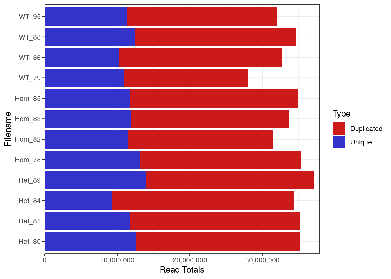
Library Sizes for each sample before any processing was undertaken.
| Version | Author | Date |
|---|---|---|
| bc12101 | Steve Ped | 2020-01-20 |
GC Content
As this was a total RNA dataset, GC content will provide a clear marker of the success of rRNA depletion. This was plotted, with all R2 reads showing a far greater spike in GC content at 81%, which is likely due to incomplete rRNA depletion. In particular, the mutant samples appeared most significantly affected raising possibility that overall GC content may be affected in these samples.
gcPlots <- list(
    r1 = plotGcContent(
        x = rawFqc[r1],
        labels = labels[r1],
        plotType = "line",
        gcType = "Transcriptome",
        species = "Drerio"
    ),
    r2 = plotGcContent(
        x = rawFqc[!r1],
        labels = labels[!r1],
        plotType = "line",
        gcType = "Transcriptome",
        species = "Drerio"
    )
)
lg <- get_legend(gcPlots$r2 + theme(legend.position = "bottom"))
plot_grid(
    plot_grid(
        r1 = gcPlots$r1 +
            ggtitle("R1: GC Distribution", subtitle = c()) +
            theme(legend.position = "none"),
        r2 = gcPlots$r2 +
            ggtitle("R2: GC Distribution", subtitle = c()) +
            theme(legend.position = "none")
    ),
    lg = lg,
    nrow = 2,
    rel_heights = c(5,2)
)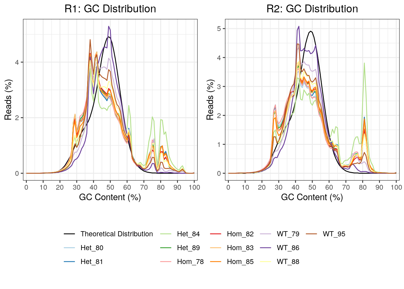
GC content for R1 and R2 reads. Notably, the R2 reads had clearer spikes in GC content above 70%
| Version | Author | Date |
|---|---|---|
| bc12101 | Steve Ped | 2020-01-20 |
gc <- getModule(rawFqc, "Per_sequence_GC")
rawGC <- gc %>%
    group_by(Filename) %>%
    mutate(Freq = Count / sum(Count)) %>%
    dplyr::filter(GC_Content > 70) %>%
    summarise(Freq = sum(Freq)) %>%
    arrange(desc(Freq)) %>%
    left_join(samples)
rawGC %>%
    ggplot(aes(sampleID, Freq, fill = reads)) +
    geom_bar(stat = "identity", position = "dodge") +
    facet_wrap(~genotype, scales = "free_x") +
    scale_y_continuous(labels = percent) +
    scale_fill_manual(values = twoCols) +
    labs(x = "Sample", y = "Percent of Total")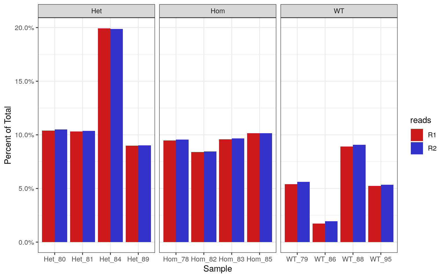
Percentages of each library which contain >70% GC. Using the known theoretical distribution, this should be 0.19% of the total library.
| Version | Author | Date |
|---|---|---|
| bc12101 | Steve Ped | 2020-01-20 |
As an alternative viewpoint, the standard deviation of observed GC frequencies from the expected GC frequencies, as obtained from the known transcriptome, were calculated. This may be a less subjective approach, which is more applicable to other datasets. Very similar patterns were seen as to those using GC% > 70.
gcDev <- gc %>%
    left_join(samples) %>%
    group_by(sampleName, sampleID) %>%
    mutate(Freq = Count / sum(Count)) %>%
    left_join(
        getGC(gcTheoretical, "Drerio", "Trans")
    ) %>%
    dplyr::rename(actual = Drerio) %>%
    mutate(res = Freq - actual) %>%
    summarise(ss = sum(res^2), n = n()) %>%
    ungroup() %>%
    mutate(sd = sqrt(ss / (n - 1)))
gcDev %>%
left_join(samples) %>%
ggplot(aes(sampleID, sd)) +
geom_bar(stat= "identity", position ="dodge") +
facet_wrap(~genotype, scales = "free_x") +
scale_fill_manual()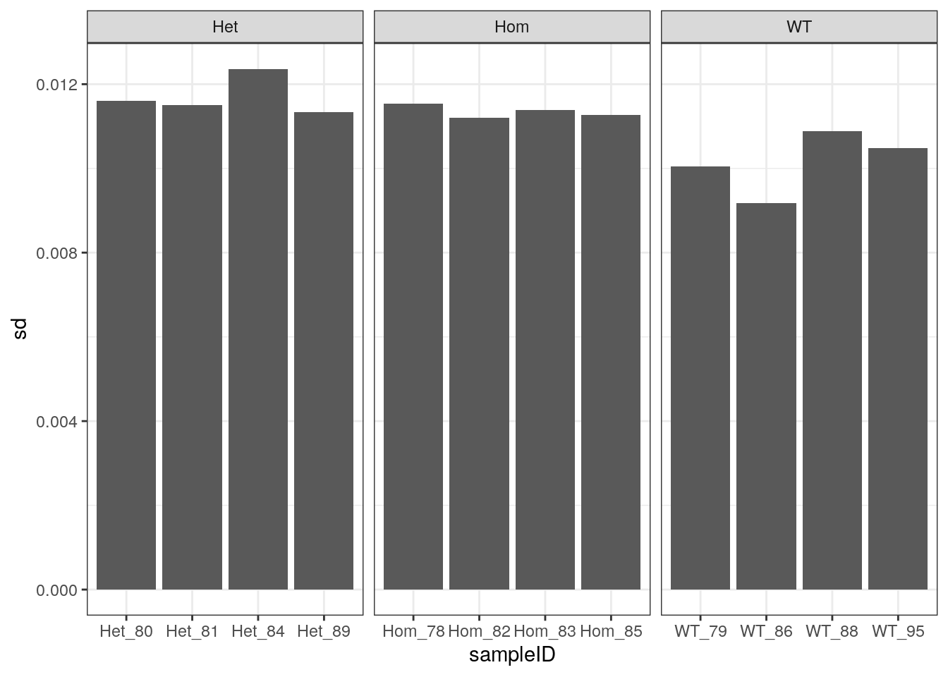
Standard deviations of observed GC frequency Vs Expected GC frequency using the theoretical GC across both sets of reads.
| Version | Author | Date |
|---|---|---|
| 68033fe | Steve Ped | 2020-01-26 |
gcDev %>%
    left_join(rawGC) %>%
    ggplot(aes(sd, Freq)) +
    geom_point() +
    geom_smooth(method = "lm") +
    labs(
        x = "SD (GC - Theoretical)",
        y = "%Library > GC70"
    )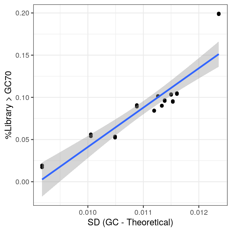
Comparison of the two measures used for assessing rRNA contamination.
| Version | Author | Date |
|---|---|---|
| 0feb548 | Steve Ped | 2020-01-28 |
Over-represented Sequences
The top 30 Overrepresented sequences were analysed using blastn and most were found to be mitochondrial rRNA sequences.
getModule(rawFqc, "Overrep") %>%
    group_by(Sequence, Possible_Source) %>%
    summarise(`Found In` = n(), `Highest Percentage` = max(Percentage)) %>%
    arrange(desc(`Highest Percentage`), desc(`Found In`)) %>%
    ungroup() %>%
    dplyr::slice(1:30) %>%
    mutate(`Highest Percentage` = percent_format(0.01)(`Highest Percentage`/100)) %>%
    pander(
        justify = "llrr",
        caption = paste(
            "*Top", nrow(.),"Overrepresented sequences.",
            "The number of samples they were found in is shown,",
            "along with the percentage of the most 'contaminated' sample.*"
            )
)| Sequence | Possible_Source | Found In | Highest Percentage |
|---|---|---|---|
| GTGGGTTCAGGTAATTAATTTAAAGCTACTTTCGTGTTTGGGCCTCTAGC | No Hit | 12 | 1.72% |
| CTGGGGGAGCGGCCGCCCCGCGGCGCCCCCTCTCGTTCCCGTCTCCGGAG | No Hit | 10 | 1.69% |
| CCGCTGTATTACTCAGGCTGCACTGCAGTGTCTATTCACAGGCGCGATCC | No Hit | 12 | 1.32% |
| GGCCCGGCGCACGTCCAGAGTCGCCGCCGCACACCGCAGCGCATCCCCCC | No Hit | 9 | 1.31% |
| CTCCTGAAAAGGTTGTATCCTTTGTTAAAGGGGCTGTACCCTCTTTAACT | No Hit | 11 | 1.11% |
| GGTTCAGGTAATTAATTTAAAGCTACTTTCGTGTTTGGGCCTCTAGCATC | No Hit | 12 | 1.09% |
| GGGGTGTACGAAGCTGAACTTTTATTCATCTCCCAGACAACCAGCTATTG | No Hit | 12 | 1.07% |
| GGCCCGGCGCACGTCCAGAGTCGCCGCCGCGCACCGCAGCGCATCCCCCC | No Hit | 10 | 1.03% |
| CGAGAGGCTCTAGTTGATATACTACGGCGTAAAGGGTGGTTAAGGAACAA | No Hit | 12 | 1.01% |
| GGGGGAGCGGCCGCCCCGCGGCGCCCCCTCTCGTTCCCGTCTCCGGAGCG | No Hit | 9 | 0.87% |
| CCTCCTTCAAGTATTGTTTCATGTTACATTTTCGTATATTCTGGGGTAGA | No Hit | 12 | 0.82% |
| CCCGCTGTATTACTCAGGCTGCACTGCAGTGTCTATTCACAGGCGCGATC | No Hit | 12 | 0.79% |
| GTTCAGGTAATTAATTTAAAGCTACTTTCGTGTTTGGGCCTCTAGCATCT | No Hit | 12 | 0.79% |
| GGGTTCAGGTAATTAATTTAAAGCTACTTTCGTGTTTGGGCCTCTAGCAT | No Hit | 12 | 0.78% |
| CGGGTCGGGTGGGTGGCCGGCATCACCGCGGACCTCGGGCGCCCTTTTGG | No Hit | 12 | 0.73% |
| GGGCCTCTAGCATCTAAAAGCGTATAACAGTTAAAGGGCCGTTTGGCTTT | No Hit | 11 | 0.68% |
| CAGTGGCGTGCGCCTGTAATCCAAGCTACTGGGAGGCTGAGGCTGGCGGA | No Hit | 11 | 0.64% |
| CGGGTCGGGTGGGTAGCCGGCATCACCGCGGACCTCGGGCGCCCTTTTGG | No Hit | 12 | 0.57% |
| CTTAGACGACCTGGTAGTCCAAGGCTCCCCCAGGAGCACCATATCGATAC | No Hit | 11 | 0.54% |
| AGCTGGGGAGATCCGCGAGAAGGGCCCGGCGCACGTCCAGAGTCGCCGCC | No Hit | 11 | 0.53% |
| GGCCTCTAGCATCTAAAAGCGTATAACAGTTAAAGGGCCGTTTGGCTTTA | No Hit | 10 | 0.53% |
| CAGCCTATTTAACTTAGGGCCAACCCGTCTCTGTGGCAATAGAGTGGGAA | No Hit | 12 | 0.51% |
| GGGTGGGTGGCCGGCATCACCGCGGACCTCGGGCGCCCTTTTGGACGTGG | No Hit | 10 | 0.50% |
| GGGAGCGGCCGCCCCGCGGCGCCCCCTCTCGTTCCCGTCTCCGGAGCGCG | No Hit | 9 | 0.49% |
| CTGGGAGATGAATAAAAGTTCAGCTTCGTACACCCCAAATTAAAAAATTA | No Hit | 10 | 0.48% |
| GCCTATTTAACTTAGGGCCAACCCGTCTCTGTGGCAATAGAGTGGGAAGA | No Hit | 12 | 0.47% |
| GGTCGGGTGGGTGGCCGGCATCACCGCGGACCTCGGGCGCCCTTTTGGAC | No Hit | 11 | 0.45% |
| CCCCCGAACCCTTCCAAGCCGAACCGGAGCCGGTCGCGGCGCACCGCCGA | No Hit | 10 | 0.45% |
| GTCGGGTGGGTGGCCGGCATCACCGCGGACCTCGGGCGCCCTTTTGGACG | No Hit | 10 | 0.43% |
| GCCCACTACGACAACGTGTTTTGTAAATTATGATCTTTATTCTCCTGAAA | No Hit | 10 | 0.43% |
Trimming
trimFqc <- list.files(
    path = "data/1_trimmedData/FastQC/",
    pattern = "zip",
    full.names = TRUE
) %>%
    FastqcDataList()
trimStats <- readTotals(rawFqc) %>%
    dplyr::rename(Raw = Total_Sequences) %>%
    left_join(readTotals(trimFqc), by = "Filename") %>%
    dplyr::rename(Trimmed = Total_Sequences) %>%
    dplyr::filter(grepl("R1", Filename)) %>%
    mutate(
        Discarded = 1 - Trimmed/Raw,
        Retained = Trimmed / Raw
    )
After adapter trimming between 4.16% and 5.08% of reads were discarded. No other improvement was noted.
Aligned Data
Trimmed reads were:
- aligned to the reference genome using
STAR 2.7.0dand summarised to each gene usingfeatureCounts. These counts were to be used for all gene-level analysis - aligned using kallisto to a modified transcriptome which contained the psen2S4Ter sequence as an ‘alternative’ transcript of psen2. This data was used for genotype checking, and assessing any GC bias in the data. Whilst transcript-level information is included for rRNA genes in the
EnsDbobject, these transcripts are excluded by default from the reference transcriptome provided by Ensembl.
Genotype Checking
cpm(kallisto$counts) %>%
    .[c("ENSDART00000006381.8", "psen2S4Ter"),] %>%
    as.data.frame() %>%
    rownames_to_column("psen2") %>%
    pivot_longer(cols = contains("kall"), names_to = "Sample", values_to = "CPM") %>%
    mutate(
        Sample = basename(Sample),
        psen2 = case_when(
            psen2 == "psen2S4Ter" ~ "S4Ter",
            psen2 != "psen2S4Ter" ~ "WT"
        )
    ) %>%
    left_join(samples, by = c("Sample" = "sampleName")) %>%
    ggplot(aes(sampleID, CPM, fill = psen2)) +
    geom_bar(stat = "identity") +
    scale_fill_manual(values = twoCols) +
    facet_wrap(~genotype, nrow = 1, scales = "free_x")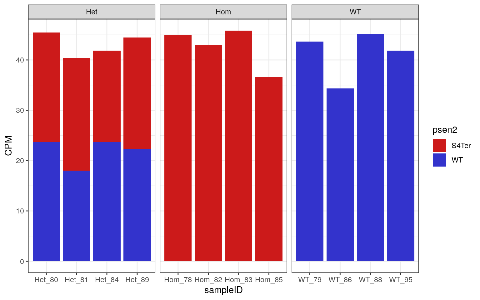
CPM obtained for both WT and S4Ter mutant transcripts of psen2
| Version | Author | Date |
|---|---|---|
| bc12101 | Steve Ped | 2020-01-20 |
As all samples demonstrated the expected expression patterns, no mislabelling was detected in this dataset.
GC Content
gcInfo <- kallisto$counts %>%
    as.data.frame() %>%
    rownames_to_column("tx_id") %>%
    dplyr::filter(
        tx_id != "psen2S4Ter"
    ) %>%
    as_tibble() %>%
    pivot_longer(
        cols = contains("kall"),
        names_to = "sampleName",
        values_to = "counts"
    ) %>%
    dplyr::filter(
        counts > 0
    ) %>%
    mutate(
        sampleName = basename(sampleName),
        tx_id_version = tx_id,
        tx_id = str_replace(tx_id, "(ENSDART[0-9]+).[0-9]+", "\\1")
    ) %>%
    left_join(
        mcols(grTrans) %>% as.data.frame()
    ) %>%
    dplyr::select(
        ends_with("id"), sampleName, counts, gc_content, length
    ) %>%
    split(f = .$sampleName) %>%
    lapply(function(x){
        DataFrame(
            gc = Rle(x$gc_content/100, x$counts),
            logLen = Rle(log10(x$length), x$counts)
        )
    }
    )
gcSummary <- gcInfo %>%
    vapply(function(x){
        c(mean(x$gc), sd(x$gc), mean(x$logLen), sd(x$logLen))
        }, numeric(4)
        ) %>%
    t() %>%
    set_colnames(
        c("mn_gc", "sd_gc", "mn_logLen", "sd_logLen")
    ) %>%
    as.data.frame() %>%
    rownames_to_column("sampleName") %>%
    as_tibble() %>%
    left_join(dplyr::filter(samples, reads == "R1")) %>%
    dplyr::select(starts_with("sample"), genotype, contains("_"))
gcCors <- rawGC %>%
dplyr::filter(reads == "R1") %>%
dplyr::select(starts_with("sample"), genotype, Freq, reads) %>%
left_join(gcSummary) %>%
left_join(gcDev) %>%
dplyr::select(Freq, mn_gc, mn_logLen, sd) %>%
cor()The initial QC steps identified an unusually large proportion of reads with >70% GC content, and noticeable deviations from the expected GC content. As such an exploration of any residual impacts this may have on the remainder of the library was performed.
A run length encoded (RLE) vector was formed for each sample taking the number of reads for each transcript as the run lengths, and both the GC content and length of each transcript as the values. Transcript lengths were transformed to the log10 scale due to the wide variety of lengths contained in the transcriptome.
From these RLEs, the mean GC and mean length was calculated for each sample, and these values were compared to the proportion of raw reads with > 70% GC, taking these values from the R1 libraries only.
- A correlation of -30% was found between the mean GC content after summarisation to transcript-level counts and the proportion of the original sequence libraries with >70% GC. This makes intuitive sense and suggests that the amount of high-GC reads in the initial libraries, as representative of incomplete rRNA removal, negatively biases the GC composition of the non-ribosomal RNA component of the library.
- A correlation of -80% was found was found between the mean transcript length of the libraries after summarisation to transcript-level counts and the proportion of the original sequence libraries with >70% GC. This is far less obvious mechanistically, but suggests that incomplete rRNA removal also biases the fragmentation or length selection process.
- Similar patterns were seen when using the standard deviations as compared to the expected values.
Given the more successful rRNA-removal in the wild-type samples, this dataset is likely to contain significant GC and Length bias which is non-biological in origin.
a <- gcSummary %>%
    left_join(rawGC) %>%
    dplyr::filter(reads == "R1") %>%
    ggplot(aes(Freq, mn_logLen)) +
    geom_point(aes(colour = genotype), size = 3) +
    geom_smooth(method = "lm") +
    scale_shape_manual(values = c(19, 1)) +
    labs(
        x = "Proportion of initial library with > 70% GC",
        y = "Mean log(length)",
        colour = "Genotype"
    )
b <- gcSummary %>%
    left_join(rawGC) %>%
    dplyr::filter(reads == "R1") %>%
    ggplot(aes(Freq, mn_gc)) +
    geom_point(aes(colour = genotype), size = 3) +
    geom_smooth(method = "lm") +
    scale_shape_manual(values = c(19, 1)) +
    scale_y_continuous(labels = percent) +
    labs(
        x = "Proportion of initial library with > 70% GC",
        y = "Mean GC Content",
        colour = "Genotype"
    )
c <- gcSummary %>%
    left_join(gcDev) %>%
    ggplot(aes(sd, mn_logLen)) +
    geom_point(aes(colour = genotype), size = 3) +
    geom_smooth(method = "lm") +
    scale_shape_manual(values = c(19, 1)) +
    scale_y_continuous(breaks = seq(3.2, 3.5, by = 0.02)) +
    labs(
        x = "SD (GC - Theoretical)",
        y = "Mean log(length)",
        colour = "Genotype"
    )
d <- gcSummary %>%
    left_join(gcDev) %>%
    ggplot(aes(sd, mn_gc)) +
    geom_point(aes(colour = genotype), size = 3) +
    geom_smooth(method = "lm") +
    scale_shape_manual(values = c(19, 1)) +
    scale_y_continuous(labels = percent) +
    labs(
        x = "SD (GC - Theoretical)",
        y = "Mean GC Content",
        colour = "Genotype"
    )
plot_grid(
    plot_grid(
        a + theme(legend.position = "none"),
        b + theme(legend.position = "none"),
        c + theme(legend.position = "none"),
        d + theme(legend.position = "none"),
        nrow = 2
    ),
    get_legend(b),
    nrow = 1,
    rel_widths = c(8,1)
)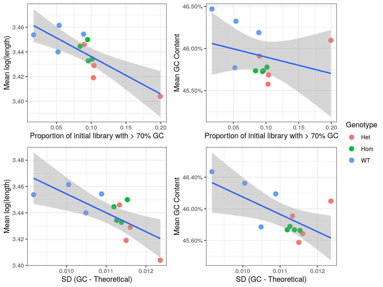
Comparison of bias introduced by incomplete rRNA removal. Regression lines are shown along with standard error bands for each comparison.
PCA
An initial PCA was performed using transcript-level counts to assess general patterns in the data. Transcripts were included if >12 reads over all libraries were allocated to that identifiers. Correlations were checked between the first three components and mean GC content (as described above), mean log10 transcript length, genotype and the proportion of the initial libraries with GC content > 70%.
The confounding of genotype and GC variability may need careful handling in this dataset.
transDGE <- kallisto$counts %>%
    set_colnames(basename(colnames(.))) %>%
    divide_by(kallisto$annotation$Overdispersion) %>%
    .[rowSums(.) > 12,] %>%
    DGEList(
        samples = tibble(
            sampleName = colnames(.)
        ) %>%
            left_join(samples) %>%
            dplyr::select(sampleName, sample = sampleID, genotype) %>%
            distinct(sampleName, .keep_all = TRUE)
    )
pca <- cpm(transDGE, log = TRUE) %>%
t() %>%
prcomp()pca$x %>%
as.data.frame() %>%
rownames_to_column("sampleName") %>%
left_join(gcSummary) %>%
as_tibble() %>%
left_join(
dplyr::filter(rawGC, reads == "R1")
) %>%
left_join(gcDev) %>%
dplyr::select(
PC1, PC2, PC3,
Mean_GC = mn_gc,
Mean_Length = mn_logLen,
Initial_GC70 = Freq,
SD = sd,
genotype
) %>%
mutate(genotype = as.numeric(as.factor(genotype))) %>%
cor() %>%
corrplot(
type = "lower",
diag = FALSE,
addCoef.col = 1, addCoefasPercent = TRUE
)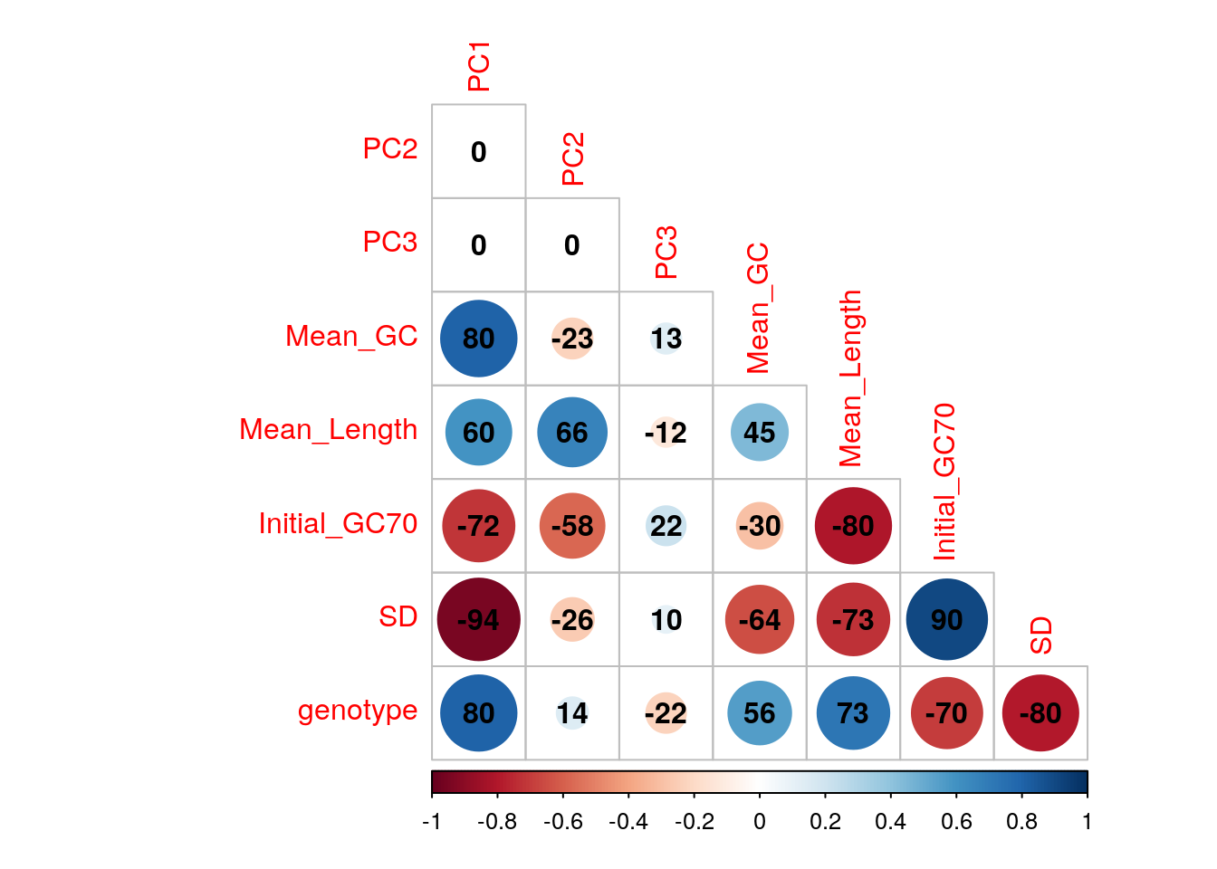
Correlations between the first three principal components and measured variables. Genotypes were converted to an ordered categorical variable for the purposes of visualisation
a <- pca$x %>%
    as.data.frame() %>%
    rownames_to_column("sampleName") %>%
    left_join(
        dplyr::filter(rawGC, reads == "R1")
    ) %>%
    as_tibble() %>%
    ggplot(aes(PC1, PC2, colour = genotype)) +
    geom_point() +
    labs(
        x = paste0("PC1 (", percent(summary(pca)$importance["Proportion of Variance","PC1"]),")"),
        y = paste0("PC2 (", percent(summary(pca)$importance["Proportion of Variance","PC2"]),")"),
        colour = "Genotype"
    )
b <- pca$x %>%
    as.data.frame() %>%
    rownames_to_column("sampleName") %>%
    left_join(gcSummary) %>%
    left_join(
        dplyr::filter(rawGC, reads == "R1")
    ) %>%
    as_tibble() %>%
    ggplot(aes(PC1, mn_gc)) +
    geom_point(aes(colour = genotype)) +
    geom_smooth(method = "lm") +
    scale_y_continuous(labels = percent) +
    labs(
        x = paste0("PC1 (", percent(summary(pca)$importance["Proportion of Variance","PC1"]),")"),
        y = "Mean GC",
        colour = "Genotype"
    )
c <- pca$x %>%
    as.data.frame() %>%
    rownames_to_column("sampleName") %>%
    left_join(gcDev) %>%
    left_join(
        rawGC %>% dplyr::filter(reads == "R1")
    ) %>%
    ggplot(aes(PC1, sd)) +
    geom_point(aes(colour = genotype)) +
    geom_smooth(method = "lm") +
    labs(
        x = paste0("PC1 (", percent(summary(pca)$importance["Proportion of Variance","PC1"]),")"),
        y = "Standard Deviation",
        colour = "Genotype"
    )
plot_grid(
    plot_grid(
        a + theme(legend.position = "none"),
        b + theme(legend.position = "none"),
        c + theme(legend.position = "none"),
        nrow = 1
    ),
    get_legend(b + theme(legend.position = "bottom")),
    nrow = 2,
    rel_heights = c(4,1)
)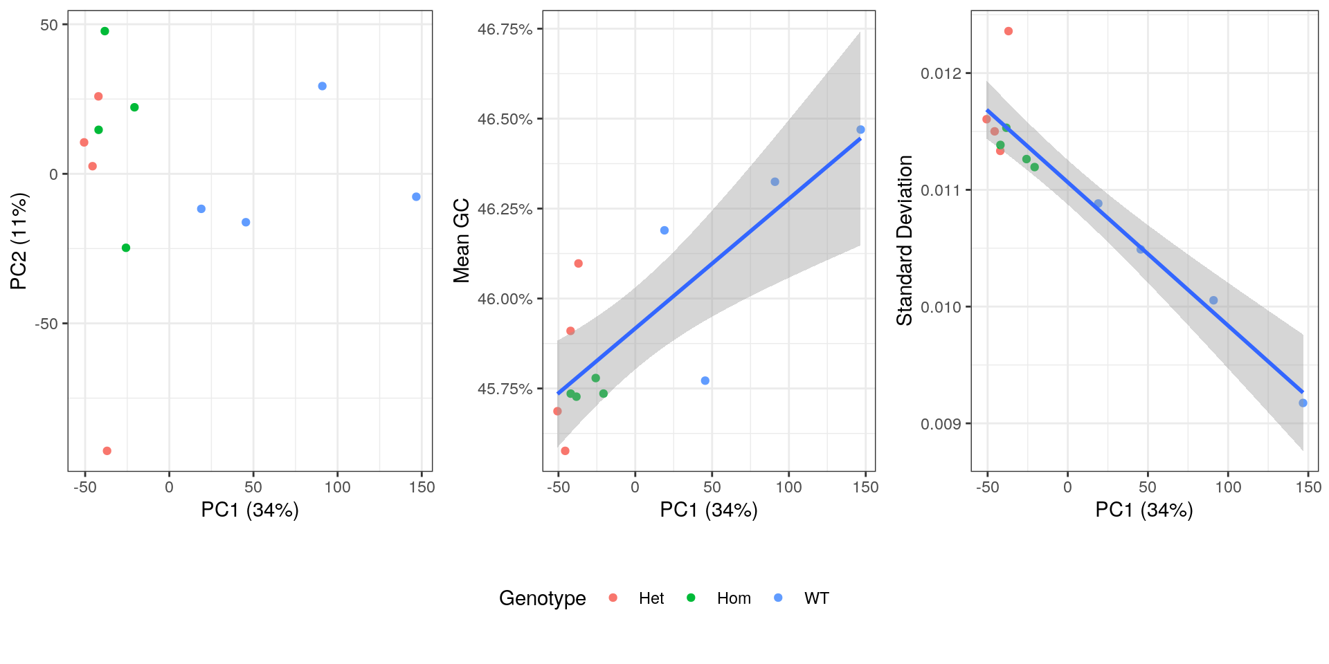
PCA plot showing genotype, mean GC content, standard deviation from theoretical and after summarisation to transcript-level.
devtools::session_info()─ Session info ───────────────────────────────────────────────────────────────
setting value
version R version 3.6.3 (2020-02-29)
os Ubuntu 18.04.4 LTS
system x86_64, linux-gnu
ui X11
language en_AU:en
collate en_AU.UTF-8
ctype en_AU.UTF-8
tz Australia/Adelaide
date 2020-04-02
─ Packages ───────────────────────────────────────────────────────────────────
package * version date lib source
AnnotationDbi * 1.48.0 2019-10-29 [2] Bioconductor
AnnotationFilter * 1.10.0 2019-10-29 [2] Bioconductor
AnnotationHub * 2.18.0 2019-10-29 [2] Bioconductor
askpass 1.1 2019-01-13 [2] CRAN (R 3.6.0)
assertthat 0.2.1 2019-03-21 [2] CRAN (R 3.6.0)
backports 1.1.5 2019-10-02 [2] CRAN (R 3.6.1)
Biobase * 2.46.0 2019-10-29 [2] Bioconductor
BiocFileCache * 1.10.2 2019-11-08 [2] Bioconductor
BiocGenerics * 0.32.0 2019-10-29 [2] Bioconductor
BiocManager 1.30.10 2019-11-16 [2] CRAN (R 3.6.1)
BiocParallel 1.20.1 2019-12-21 [2] Bioconductor
BiocVersion 3.10.1 2019-06-06 [2] Bioconductor
biomaRt 2.42.0 2019-10-29 [2] Bioconductor
Biostrings 2.54.0 2019-10-29 [2] Bioconductor
bit 1.1-15.2 2020-02-10 [2] CRAN (R 3.6.2)
bit64 0.9-7 2017-05-08 [2] CRAN (R 3.6.0)
bitops 1.0-6 2013-08-17 [2] CRAN (R 3.6.0)
blob 1.2.1 2020-01-20 [2] CRAN (R 3.6.2)
broom 0.5.4 2020-01-27 [2] CRAN (R 3.6.2)
callr 3.4.2 2020-02-12 [2] CRAN (R 3.6.2)
cellranger 1.1.0 2016-07-27 [2] CRAN (R 3.6.0)
cli 2.0.1 2020-01-08 [2] CRAN (R 3.6.2)
cluster 2.1.0 2019-06-19 [2] CRAN (R 3.6.1)
colorspace 1.4-1 2019-03-18 [2] CRAN (R 3.6.0)
corrplot * 0.84 2017-10-16 [2] CRAN (R 3.6.0)
cowplot * 1.0.0 2019-07-11 [2] CRAN (R 3.6.1)
crayon 1.3.4 2017-09-16 [2] CRAN (R 3.6.0)
curl 4.3 2019-12-02 [2] CRAN (R 3.6.2)
data.table 1.12.8 2019-12-09 [2] CRAN (R 3.6.2)
DBI 1.1.0 2019-12-15 [2] CRAN (R 3.6.2)
dbplyr * 1.4.2 2019-06-17 [2] CRAN (R 3.6.0)
DelayedArray 0.12.2 2020-01-06 [2] Bioconductor
desc 1.2.0 2018-05-01 [2] CRAN (R 3.6.0)
devtools 2.2.2 2020-02-17 [2] CRAN (R 3.6.2)
digest 0.6.25 2020-02-23 [2] CRAN (R 3.6.2)
dplyr * 0.8.4 2020-01-31 [2] CRAN (R 3.6.2)
edgeR * 3.28.1 2020-02-26 [2] Bioconductor
ellipsis 0.3.0 2019-09-20 [2] CRAN (R 3.6.1)
ensembldb * 2.10.2 2019-11-20 [2] Bioconductor
evaluate 0.14 2019-05-28 [2] CRAN (R 3.6.0)
FactoMineR 2.2 2020-02-05 [2] CRAN (R 3.6.2)
fansi 0.4.1 2020-01-08 [2] CRAN (R 3.6.2)
farver 2.0.3 2020-01-16 [2] CRAN (R 3.6.2)
fastmap 1.0.1 2019-10-08 [2] CRAN (R 3.6.1)
flashClust 1.01-2 2012-08-21 [2] CRAN (R 3.6.1)
forcats * 0.4.0 2019-02-17 [2] CRAN (R 3.6.0)
fs 1.3.1 2019-05-06 [2] CRAN (R 3.6.0)
generics 0.0.2 2018-11-29 [2] CRAN (R 3.6.0)
GenomeInfoDb * 1.22.0 2019-10-29 [2] Bioconductor
GenomeInfoDbData 1.2.2 2019-11-21 [2] Bioconductor
GenomicAlignments 1.22.1 2019-11-12 [2] Bioconductor
GenomicFeatures * 1.38.2 2020-02-15 [2] Bioconductor
GenomicRanges * 1.38.0 2019-10-29 [2] Bioconductor
ggdendro 0.1-20 2016-04-27 [2] CRAN (R 3.6.0)
ggplot2 * 3.2.1 2019-08-10 [2] CRAN (R 3.6.1)
ggrepel 0.8.1 2019-05-07 [2] CRAN (R 3.6.0)
git2r 0.26.1 2019-06-29 [2] CRAN (R 3.6.1)
glue 1.3.1 2019-03-12 [2] CRAN (R 3.6.0)
gtable 0.3.0 2019-03-25 [2] CRAN (R 3.6.0)
haven 2.2.0 2019-11-08 [2] CRAN (R 3.6.1)
highr 0.8 2019-03-20 [2] CRAN (R 3.6.0)
hms 0.5.3 2020-01-08 [2] CRAN (R 3.6.2)
htmltools 0.4.0 2019-10-04 [2] CRAN (R 3.6.1)
htmlwidgets 1.5.1 2019-10-08 [2] CRAN (R 3.6.1)
httpuv 1.5.2 2019-09-11 [2] CRAN (R 3.6.1)
httr 1.4.1 2019-08-05 [2] CRAN (R 3.6.1)
hwriter 1.3.2 2014-09-10 [2] CRAN (R 3.6.0)
interactiveDisplayBase 1.24.0 2019-10-29 [2] Bioconductor
IRanges * 2.20.2 2020-01-13 [2] Bioconductor
jpeg 0.1-8.1 2019-10-24 [2] CRAN (R 3.6.1)
jsonlite 1.6.1 2020-02-02 [2] CRAN (R 3.6.2)
kableExtra 1.1.0 2019-03-16 [2] CRAN (R 3.6.1)
knitr 1.28 2020-02-06 [2] CRAN (R 3.6.2)
labeling 0.3 2014-08-23 [2] CRAN (R 3.6.0)
later 1.0.0 2019-10-04 [2] CRAN (R 3.6.1)
lattice 0.20-40 2020-02-19 [4] CRAN (R 3.6.2)
latticeExtra 0.6-29 2019-12-19 [2] CRAN (R 3.6.2)
lazyeval 0.2.2 2019-03-15 [2] CRAN (R 3.6.0)
leaps 3.1 2020-01-16 [2] CRAN (R 3.6.2)
lifecycle 0.1.0 2019-08-01 [2] CRAN (R 3.6.1)
limma * 3.42.2 2020-02-03 [2] Bioconductor
locfit 1.5-9.1 2013-04-20 [2] CRAN (R 3.6.0)
lubridate 1.7.4 2018-04-11 [2] CRAN (R 3.6.0)
magrittr * 1.5 2014-11-22 [2] CRAN (R 3.6.0)
MASS 7.3-51.5 2019-12-20 [4] CRAN (R 3.6.2)
Matrix 1.2-18 2019-11-27 [2] CRAN (R 3.6.1)
matrixStats 0.55.0 2019-09-07 [2] CRAN (R 3.6.1)
memoise 1.1.0 2017-04-21 [2] CRAN (R 3.6.0)
mime 0.9 2020-02-04 [2] CRAN (R 3.6.2)
modelr 0.1.6 2020-02-22 [2] CRAN (R 3.6.2)
munsell 0.5.0 2018-06-12 [2] CRAN (R 3.6.0)
ngsReports * 1.1.2 2019-10-16 [1] Bioconductor
nlme 3.1-144 2020-02-06 [4] CRAN (R 3.6.2)
openssl 1.4.1 2019-07-18 [2] CRAN (R 3.6.1)
pander * 0.6.3 2018-11-06 [2] CRAN (R 3.6.0)
pillar 1.4.3 2019-12-20 [2] CRAN (R 3.6.2)
pkgbuild 1.0.6 2019-10-09 [2] CRAN (R 3.6.1)
pkgconfig 2.0.3 2019-09-22 [2] CRAN (R 3.6.1)
pkgload 1.0.2 2018-10-29 [2] CRAN (R 3.6.0)
plotly 4.9.2 2020-02-12 [2] CRAN (R 3.6.2)
plyr 1.8.5 2019-12-10 [2] CRAN (R 3.6.2)
png 0.1-7 2013-12-03 [2] CRAN (R 3.6.0)
prettyunits 1.1.1 2020-01-24 [2] CRAN (R 3.6.2)
processx 3.4.2 2020-02-09 [2] CRAN (R 3.6.2)
progress 1.2.2 2019-05-16 [2] CRAN (R 3.6.0)
promises 1.1.0 2019-10-04 [2] CRAN (R 3.6.1)
ProtGenerics 1.18.0 2019-10-29 [2] Bioconductor
ps 1.3.2 2020-02-13 [2] CRAN (R 3.6.2)
purrr * 0.3.3 2019-10-18 [2] CRAN (R 3.6.1)
R6 2.4.1 2019-11-12 [2] CRAN (R 3.6.1)
rappdirs 0.3.1 2016-03-28 [2] CRAN (R 3.6.0)
RColorBrewer 1.1-2 2014-12-07 [2] CRAN (R 3.6.0)
Rcpp 1.0.3 2019-11-08 [2] CRAN (R 3.6.1)
RCurl 1.98-1.1 2020-01-19 [2] CRAN (R 3.6.2)
readr * 1.3.1 2018-12-21 [2] CRAN (R 3.6.0)
readxl 1.3.1 2019-03-13 [2] CRAN (R 3.6.0)
remotes 2.1.1 2020-02-15 [2] CRAN (R 3.6.2)
reprex 0.3.0 2019-05-16 [2] CRAN (R 3.6.0)
reshape2 1.4.3 2017-12-11 [2] CRAN (R 3.6.0)
rhdf5 2.30.1 2019-11-26 [2] Bioconductor
Rhdf5lib 1.8.0 2019-10-29 [2] Bioconductor
rlang 0.4.4 2020-01-28 [2] CRAN (R 3.6.2)
rmarkdown 2.1 2020-01-20 [2] CRAN (R 3.6.2)
rprojroot 1.3-2 2018-01-03 [2] CRAN (R 3.6.0)
Rsamtools 2.2.3 2020-02-23 [2] Bioconductor
RSQLite 2.2.0 2020-01-07 [2] CRAN (R 3.6.2)
rstudioapi 0.11 2020-02-07 [2] CRAN (R 3.6.2)
rtracklayer 1.46.0 2019-10-29 [2] Bioconductor
rvest 0.3.5 2019-11-08 [2] CRAN (R 3.6.1)
S4Vectors * 0.24.3 2020-01-18 [2] Bioconductor
scales * 1.1.0 2019-11-18 [2] CRAN (R 3.6.1)
scatterplot3d 0.3-41 2018-03-14 [2] CRAN (R 3.6.1)
sessioninfo 1.1.1 2018-11-05 [2] CRAN (R 3.6.0)
shiny 1.4.0 2019-10-10 [2] CRAN (R 3.6.1)
ShortRead 1.44.3 2020-02-03 [2] Bioconductor
stringi 1.4.6 2020-02-17 [2] CRAN (R 3.6.2)
stringr * 1.4.0 2019-02-10 [2] CRAN (R 3.6.0)
SummarizedExperiment 1.16.1 2019-12-19 [2] Bioconductor
testthat 2.3.1 2019-12-01 [2] CRAN (R 3.6.1)
tibble * 2.1.3 2019-06-06 [2] CRAN (R 3.6.0)
tidyr * 1.0.2 2020-01-24 [2] CRAN (R 3.6.2)
tidyselect 1.0.0 2020-01-27 [2] CRAN (R 3.6.2)
tidyverse * 1.3.0 2019-11-21 [2] CRAN (R 3.6.1)
truncnorm 1.0-8 2018-02-27 [2] CRAN (R 3.6.0)
usethis 1.5.1 2019-07-04 [2] CRAN (R 3.6.1)
vctrs 0.2.3 2020-02-20 [2] CRAN (R 3.6.2)
viridisLite 0.3.0 2018-02-01 [2] CRAN (R 3.6.0)
webshot 0.5.2 2019-11-22 [2] CRAN (R 3.6.1)
whisker 0.4 2019-08-28 [2] CRAN (R 3.6.1)
withr 2.1.2 2018-03-15 [2] CRAN (R 3.6.0)
workflowr * 1.6.0 2019-12-19 [2] CRAN (R 3.6.2)
xfun 0.12 2020-01-13 [2] CRAN (R 3.6.2)
XML 3.99-0.3 2020-01-20 [2] CRAN (R 3.6.2)
xml2 1.2.2 2019-08-09 [2] CRAN (R 3.6.1)
xtable 1.8-4 2019-04-21 [2] CRAN (R 3.6.0)
XVector 0.26.0 2019-10-29 [2] Bioconductor
yaml 2.2.1 2020-02-01 [2] CRAN (R 3.6.2)
zlibbioc 1.32.0 2019-10-29 [2] Bioconductor
zoo 1.8-7 2020-01-10 [2] CRAN (R 3.6.2)
[1] /home/steveped/R/x86_64-pc-linux-gnu-library/3.6
[2] /usr/local/lib/R/site-library
[3] /usr/lib/R/site-library
[4] /usr/lib/R/library