Differential Expression
Steve Pederson
02 April, 2020
Last updated: 2020-04-02
Checks: 7 0
Knit directory: 20170327_Psen2S4Ter_RNASeq/
This reproducible R Markdown analysis was created with workflowr (version 1.6.0). The Checks tab describes the reproducibility checks that were applied when the results were created. The Past versions tab lists the development history.
Great! Since the R Markdown file has been committed to the Git repository, you know the exact version of the code that produced these results.
Great job! The global environment was empty. Objects defined in the global environment can affect the analysis in your R Markdown file in unknown ways. For reproduciblity it’s best to always run the code in an empty environment.
The command set.seed(20200119) was run prior to running the code in the R Markdown file. Setting a seed ensures that any results that rely on randomness, e.g. subsampling or permutations, are reproducible.
Great job! Recording the operating system, R version, and package versions is critical for reproducibility.
Nice! There were no cached chunks for this analysis, so you can be confident that you successfully produced the results during this run.
Great job! Using relative paths to the files within your workflowr project makes it easier to run your code on other machines.
Great! You are using Git for version control. Tracking code development and connecting the code version to the results is critical for reproducibility. The version displayed above was the version of the Git repository at the time these results were generated.
Note that you need to be careful to ensure that all relevant files for the analysis have been committed to Git prior to generating the results (you can use wflow_publish or wflow_git_commit). workflowr only checks the R Markdown file, but you know if there are other scripts or data files that it depends on. Below is the status of the Git repository when the results were generated:
Ignored files:
    Ignored:    .Rhistory
    Ignored:    .Rproj.user/

Untracked files:
    Untracked:  basic_sample_checklist.txt
    Untracked:  experiment_paired_fastq_spreadsheet_template.txt

Unstaged changes:
    Modified:   analysis/_site.yml
    Modified:   data/cpmPostNorm.rds
    Modified:   data/dgeList.rds
    Modified:   data/fit.rds
    Modified:   output/psen2HomVsHet.csv
    Modified:   output/psen2VsWT.csv

Staged changes:
    Modified:   analysis/_site.yml
Note that any generated files, e.g. HTML, png, CSS, etc., are not included in this status report because it is ok for generated content to have uncommitted changes.
These are the previous versions of the R Markdown and HTML files. If you’ve configured a remote Git repository (see ?wflow_git_remote), click on the hyperlinks in the table below to view them.
| File | Version | Author | Date | Message |
|---|---|---|---|---|
| Rmd | e928a97 | Steve Ped | 2020-04-02 | Corrected original filtering |
| html | bad81c1 | Steve Ped | 2020-03-05 | Updated MutVsWt UpSet plots for KEGG/HALLMARK |
| Rmd | ba80e5e | Steve Ped | 2020-03-05 | Corrected exports |
| Rmd | 381e5de | Steve Ped | 2020-03-04 | Fixed file import |
| Rmd | 2a1a66d | Steve Ped | 2020-03-04 | Corrected file path |
| Rmd | f75f82a | Steve Ped | 2020-03-04 | Added post-CQN PCA |
| html | 86ffa07 | Steve Ped | 2020-02-20 | Updated saample layout figure |
| html | 876e40f | Steve Ped | 2020-02-17 | Compiled after minor corrections |
| html | 68033fe | Steve Ped | 2020-01-26 | Corrected chunk labels after publishing DE analysis |
| Rmd | 25922d6 | Steve Ped | 2020-01-26 | Added first pass of enrichment |
| Rmd | 96d8cc7 | Steve Ped | 2020-01-25 | Compiled after data export & added compression to output |
| html | 96d8cc7 | Steve Ped | 2020-01-25 | Compiled after data export & added compression to output |
| Rmd | 07a6053 | Steve Ped | 2020-01-25 | Corrected paths |
| Rmd | 09180e5 | Steve Ped | 2020-01-25 | Added data export |
| Rmd | fca554f | Steve Ped | 2020-01-25 | Tweaked explanations & labels |
| Rmd | be95a60 | Steve Ped | 2020-01-25 | Finished first pass of DE Analysis |
| html | be95a60 | Steve Ped | 2020-01-25 | Finished first pass of DE Analysis |
| html | f04bb47 | Steve Ped | 2020-01-25 | Minor typos |
| Rmd | 7251bd2 | Steve Ped | 2020-01-25 | Tweaks |
| Rmd | 7fea156 | Steve Ped | 2020-01-25 | Added rRNA checks & heatmaps |
| html | 9bff516 | Steve Ped | 2020-01-24 | Added analysis without CQN |
| Rmd | 7b680b2 | Steve Ped | 2020-01-24 | Added analysis without CQN |
| html | 95ccc90 | Steve Ped | 2020-01-22 | Compiled DE so far |
| Rmd | 1858f49 | Steve Ped | 2020-01-22 | Started presenting actual DE genes |
| html | 1858f49 | Steve Ped | 2020-01-22 | Started presenting actual DE genes |
| Rmd | 10a285b | Steve Ped | 2020-01-22 | Expanded description in index and tried reusing an image |
| html | 10a285b | Steve Ped | 2020-01-22 | Expanded description in index and tried reusing an image |
| html | aabb570 | Steve Ped | 2020-01-21 | Rebuilt to get rid of warnings |
| Rmd | 71b8832 | Steve Ped | 2020-01-21 | Added DE QC for GC bias |
| html | 71b8832 | Steve Ped | 2020-01-21 | Added DE QC for GC bias |
| Rmd | e825637 | Steve Ped | 2020-01-21 | Minor updates to DE plots |
| html | 01512da | Steve Ped | 2020-01-21 | Added initial DE analysis to index |
| Rmd | fbb6242 | Steve Ped | 2020-01-21 | Paused DE analysis |
| Rmd | c560637 | Steve Ped | 2020-01-20 | Started DE analysis |
Setup
library(ngsReports)
library(tidyverse)
library(magrittr)
library(edgeR)
library(AnnotationHub)
library(ensembldb)
library(scales)
library(pander)
library(cqn)
library(ggrepel)
library(pheatmap)
library(RColorBrewer)
if (interactive()) setwd(here::here())
theme_set(theme_bw())
panderOptions("big.mark", ",")
panderOptions("table.split.table", Inf)
panderOptions("table.style", "rmarkdown")Annotations
ah <- AnnotationHub() %>%
  subset(species == "Danio rerio") %>%
  subset(rdataclass == "EnsDb")
ensDb <- ah[["AH74989"]]
grTrans <- transcripts(ensDb)
trLengths <- exonsBy(ensDb, "tx") %>%
width() %>%
vapply(sum, integer(1))
mcols(grTrans)$length <- trLengths[names(grTrans)]gcGene <- grTrans %>%
mcols() %>%
as.data.frame() %>%
dplyr::select(gene_id, tx_id, gc_content, length) %>%
as_tibble() %>%
group_by(gene_id) %>%
summarise(
gc_content = sum(gc_content*length) / sum(length),
length = ceiling(median(length))
)
grGenes <- genes(ensDb)
mcols(grGenes) %<>%
as.data.frame() %>%
left_join(gcGene) %>%
as.data.frame() %>%
DataFrame()Similarly to the Quality Assessment steps, GRanges objects were formed at the gene and transcript levels, to enable estimation of GC content and length for each transcript and gene. GC content and transcript length are available for each transcript, and for gene-level estimates, GC content was taken as the sum of all GC bases divided by the sum of all transcript lengths, effectively averaging across all transcripts. Gene length was defined as the median transcript length.
samples <- read_csv("data/samples.csv") %>%
  distinct(sampleName, .keep_all = TRUE) %>%
  dplyr::select(sample = sampleName, sampleID, genotype) %>%
  mutate(
    genotype = factor(genotype, levels = c("WT", "Het", "Hom")),
    mutant = genotype %in% c("Het", "Hom"),
    homozygous = genotype == "Hom"
  )
genoCols <- samples$genotype %>%
  levels() %>%
  length() %>%
  brewer.pal("Set1") %>%
  setNames(levels(samples$genotype))
Sample metadata was also loaded, with only the sampleID and genotype being retained. All other fields were considered irrelevant.
Count Data
minCPM <- 1.5
minSamples <- 4
dgeList <- file.path("data", "2_alignedData", "featureCounts", "genes.out") %>%
  read_delim(delim = "\t") %>%
  set_names(basename(names(.))) %>%
  as.data.frame() %>%
  column_to_rownames("Geneid") %>%
  as.matrix() %>%
  set_colnames(str_remove(colnames(.), "Aligned.sortedByCoord.out.bam")) %>%
  .[rowSums(cpm(.) >= minCPM) >= minSamples,] %>%
  DGEList(
    samples = tibble(sample = colnames(.)) %>%
      left_join(samples),
    genes = grGenes[rownames(.)] %>%
      as.data.frame() %>%
      dplyr::select(
        chromosome = seqnames, start, end,
        gene_id, gene_name, gene_biotype, description,
        entrezid, gc_content, length
      )
  ) %>%
  .[!grepl("rRNA", .$genes$gene_biotype),] %>%
  calcNormFactors()
Gene-level count data as output by featureCounts, was loaded and formed into a DGEList object. During this process, genes were removed if:
- They were not considered as detectable (CPM < 1.5 in > 8 samples). This translates to > 18 reads assigned a gene in all samples from one or more of the genotype groups
- The
gene_biotypewas any type ofrRNA.
These filtering steps returned gene-level counts for 16,021 genes, with total library sizes between 11,842,836 and 16,988,116 reads assigned to genes. It was noted that these library sizes were about 1.5-fold larger than the transcript-level counts used for the QA steps.
cpm(dgeList, log = TRUE) %>%
  as.data.frame() %>%
  pivot_longer(
    cols = everything(),
    names_to = "sample",
    values_to = "logCPM"
  ) %>%
  split(f = .$sample) %>%
  lapply(function(x){
    d <- density(x$logCPM)
    tibble(
      sample = unique(x$sample),
      x = d$x,
      y = d$y
    )
  }) %>%
  bind_rows() %>%
  left_join(samples) %>%
  ggplot(aes(x, y, colour = genotype, group = sample)) +
  geom_line() +
  scale_colour_manual(
    values = genoCols
  ) +
  labs(
    x = "logCPM",
    y = "Density",
    colour = "Genotype"
  )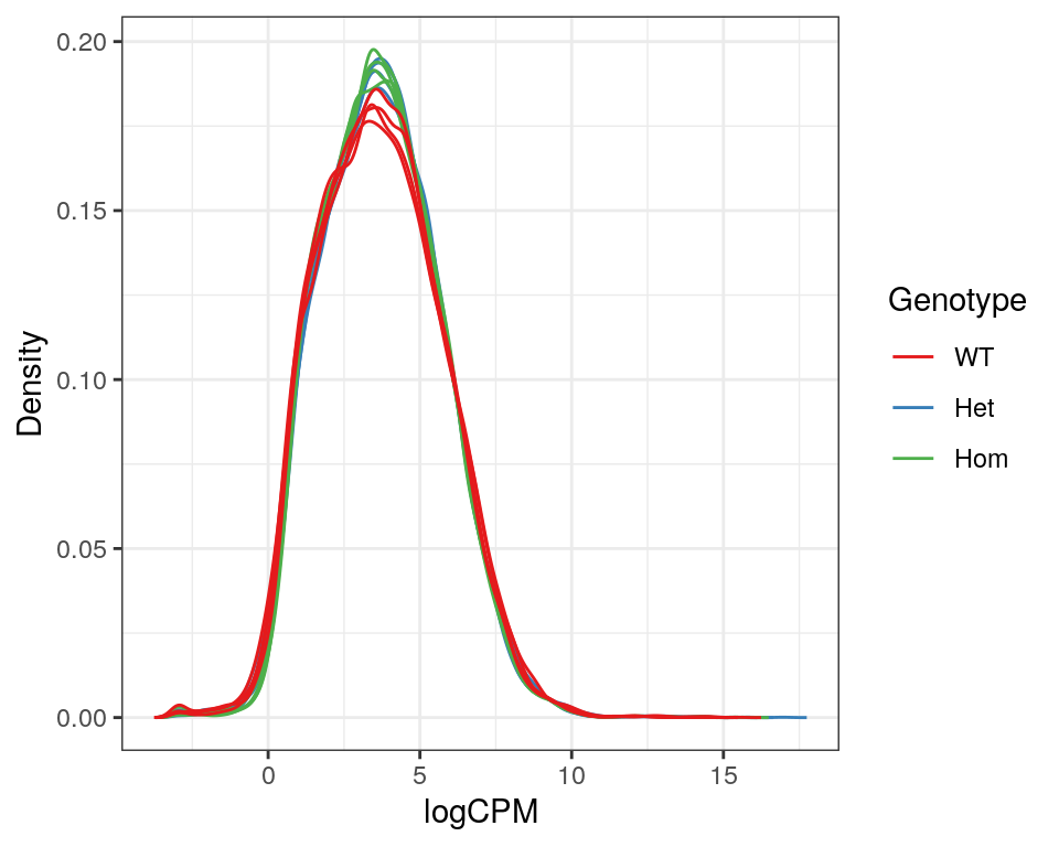
Expression density plots for all samples after filtering, showing logCPM values.
Additional Functions
contLabeller <- as_labeller(
  c(
    HetVsWT = "S4Ter/+ Vs +/+",
    HomVsWT = "S4Ter/S4Ter Vs +/+",
    HomVsHet = "S4Ter/S4Ter Vs S4Ter/+",
    Hom = "S4Ter/S4Ter",
    Het = "S4Ter/+",
    WT = "+/+",
    mutant = "S4Ter Vs WT",
    homozygous = "S4Ter/S4Ter Vs S4Ter/+"
  )
)
geneLabeller <- structure(grGenes$gene_name, names = grGenes$gene_id) %>%
  as_labeller()
Labeller functions for genotypes, contrasts and gene names were additionally defined for simpler plotting using ggplot2.
Correlations with rRNA contaminants
In order to asses the impact of the potential rRNA contaminant, correlations between the initial estimate of contamination and each gene’s expression pattern were also investigated. Conceptually, genes which are highly correlated with rRNA may be physically associated with these complexes. Similary, genes with high negative correlations may be actively selected against in the presence of rRNA complexes.
rawFqc <- list.files(
  path = "data/0_rawData/FastQC/",
  pattern = "zip",
  full.names = TRUE
) %>%
  FastqcDataList()
gc <- getModule(rawFqc, "Per_sequence_GC") %>%
  group_by(Filename) %>%
  mutate(Freq = Count / sum(Count)) %>%
  ungroup()
rawGC <- gc %>%
  dplyr::filter(GC_Content > 70) %>%
  group_by(Filename) %>%
  summarise(Freq = sum(Freq)) %>%
  arrange(desc(Freq)) %>%
  mutate(sample = str_remove(Filename, "_R[12].fastq.gz")) %>%
  group_by(sample) %>%
  summarise(Freq = mean(Freq)) %>%
  left_join(samples)
riboVec <- structure(rawGC$Freq, names = rawGC$sample)
riboCors <- cpm(dgeList, log = TRUE) %>%
apply(1, function(x){
cor(x, riboVec[names(x)])
})Analysis
Initial PCA
pca <- dgeList %>%
  cpm(log = TRUE) %>%
  t() %>%
  prcomp()
pcaVars <- percent_format(0.1)(summary(pca)$importance["Proportion of Variance",])
pca$x %>%
as.data.frame() %>%
rownames_to_column("sample") %>%
left_join(samples) %>%
as_tibble() %>%
ggplot(aes(PC1, PC2, colour = genotype, fill = genotype)) +
geom_point() +
geom_text_repel(aes(label = sampleID), show.legend = FALSE) +
stat_ellipse(geom = "polygon", alpha = 0.05, show.legend = FALSE) +
guides(fill = FALSE) +
scale_colour_manual(
values = genoCols
) +
labs(
x = paste0("PC1 (", pcaVars[["PC1"]], ")"),
y = paste0("PC2 (", pcaVars[["PC2"]], ")"),
colour = "Genotype"
)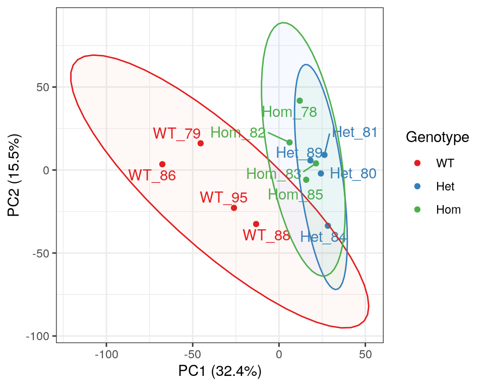
PCA of gene-level counts.
A Principal Component Analysis (PCA) was also performed using logCPM values from each sample. Both mutant genotypes appear to cluster together, however it has previously been noted that GC content appears to track closely with PC1, as a result of variable rRNA removal.
Model Description

The initial expectation was to perform three pairwise comparisons as described in the above figure. However, given there was a strong similarity between mutants, the model matrix was defined as containing an intercept (i.e. baseline expression in wild-type), with additional columns defining presence of any mutant alleles, and the final column capturing the difference between mutants. This avoids any issues with the use of hard cutoffs when combing lists, such as would occur when comparing separate results from both mutant genotypes against wild-type samples.
d <- model.matrix(~mutant + homozygous, data = dgeList$samples) %>%
  set_colnames(str_remove(colnames(.), "TRUE"))
pheatmap(
d,
cluster_cols = FALSE,
cluster_rows = FALSE,
color = c("white", "grey50"),
annotation_row = dgeList$samples["genotype"],
annotation_colors = list(genotype = genoCols),
legend = FALSE
)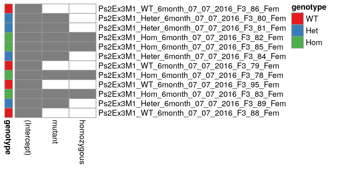
Visualisation of the design matrix
| Version | Author | Date |
|---|---|---|
| 7251bd2 | Steve Ped | 2020-01-25 |
Conditional Quantile Normalisation
As GC content and length was noted as being of concern for this dataset, conditional-quantile normalisation was performed using the cqn package. This adds a gene and sample-level offset for each count which takes into account any systemic bias, such as that identified previously as an artefact of variable rRNA removal. The resultant glm.offset values were added to the original DGEList object, and all dispersion estimates were calculated.
gcCqn <- cqn(
  counts = dgeList$counts,
  x = dgeList$genes$gc_content,
  lengths = dgeList$genes$length,
  sizeFactors = dgeList$samples$lib.size
)
par(mfrow = c(1, 2))
cqnplot(gcCqn, n = 1, xlab = "GC Content", col = genoCols)
cqnplot(gcCqn, n = 2, xlab = "Length", col = genoCols)
legend("bottomright", legend = levels(samples$genotype), col = genoCols, lty = 1)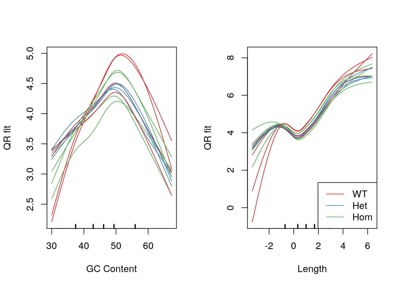
Model fits for GC content and gene length under the CQN model. Genotype-specific effects are clearly visible.
par(mfrow = c(1, 1))dgeList$offset <- gcCqn$glm.offset
dgeList %<>% estimateDisp(design = d)PCA After Normalisation
cpmPostNorm <- gcCqn %>%
  with(y + offset)
pcaPost <- cpmPostNorm %>%
t() %>%
prcomp()
pcaVars <- percent_format(0.1)(summary(pcaPost)$importance["Proportion of Variance",])pcaPost$x %>%
as.data.frame() %>%
rownames_to_column("sample") %>%
left_join(samples) %>%
as_tibble() %>%
ggplot(aes(PC1, PC2, colour = genotype, fill = genotype)) +
geom_point() +
geom_text_repel(aes(label = sampleID), show.legend = FALSE) +
stat_ellipse(geom = "polygon", alpha = 0.05, show.legend = FALSE) +
guides(fill = FALSE) +
scale_colour_manual(
values = genoCols
) +
labs(
x = paste0("PC1 (", pcaVars[["PC1"]], ")"),
y = paste0("PC2 (", pcaVars[["PC2"]], ")"),
colour = "Genotype"
)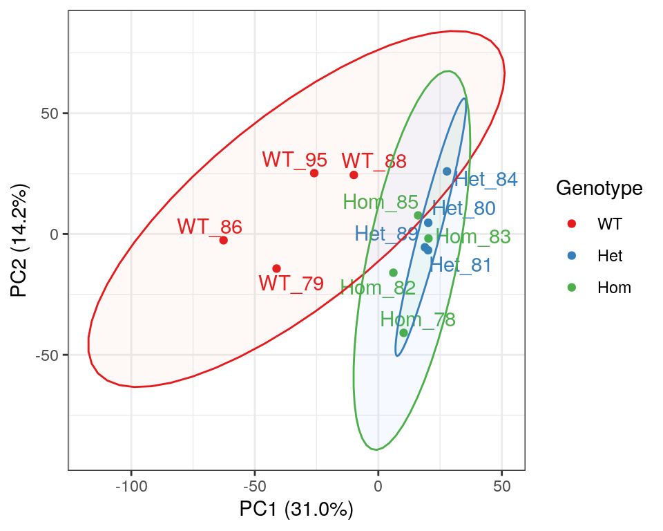
PCA of gene-level counts after conditional quantile normalisation.
| Version | Author | Date |
|---|---|---|
| 7fe1505 | Steve Ped | 2020-03-05 |
After conditional quantile normalisation, a second PCA analysis was performed in order to check for improvement in group separation. However, there appeared to minimal improvement at this level, with PC1 still only accounting for 31.0% of the variability.
Model Fitting
minLfc <- log2(2)
alpha <- 0.01
fit <- glmFit(dgeList)
topTables <- colnames(d)[2:3] %>%
  sapply(function(x){
    glmLRT(fit, coef = x) %>%
      topTags(n = Inf) %>%
      .[["table"]] %>%
      as_tibble() %>%
      arrange(PValue) %>%
      dplyr::select(
        gene_id, gene_name, logFC, logCPM, PValue, FDR, everything()
      ) %>%
      mutate(
        coef = x,
        bonfP = p.adjust(PValue, "bonf"),
        DE = case_when(
          bonfP < alpha ~ TRUE,
          FDR < alpha & abs(logFC) > minLfc ~ TRUE
        ),
        DE = ifelse(is.na(DE), FALSE, DE)
      )
  }, simplify = FALSE)
Models were fit using the negative-binomial approaches of glmFit(). Top Tables were then obtained using likelihood-ratio tests in glmLRT(). These test the standard \(H_0\) that the true value of the estimated model coefficient is zero. These model coefficients effectively estimate:
- the effect of the presence of a mutation, and
- the difference in heterozygous and heterozygous mutants
For enrichment testing, genes were initially considered to be DE using:
- A Bonferroni-adjusted p-value < 0.01
- An FDR-adjusted p-value < 0.01 along with an estimated logFC outside of the range \(\pm \log_2(2)\).
As fewer genes were detected in the comparisons between homozygous and heterozygous mutants, a simple FDR of 0.05 was subsequently chosen for this comparison.
topTables$homozygous %<>%
  mutate(DE = FDR < 0.05)
Using these criteria, the following initial DE gene-sets were defined:
topTables %>%
  lapply(dplyr::filter, DE) %>%
  vapply(nrow, integer(1)) %>%
  set_names(
    case_when(
      names(.) == "mutant" ~ "psen2 mutant",
      names(.) == "homozygous" ~ "HomVsHet"
    )
  ) %>%
pander()| psen2 mutant | HomVsHet |
|---|---|
| 599 | 7 |
deCols <- c(
  `FALSE` = rgb(0.5, 0.5, 0.5, 0.4),
  `TRUE` = rgb(1, 0, 0, 0.7)
)
Model Checking
Checks for rRNA impacts
Given the previously identified concerns about variable rRNA removal, correlations were calculated between each gene’s expression values and the proportion of the raw libraries with > 70% GC. Those with the strongest +ve correlation, and for which the FDR is < 0.01 are shown below.
Most notably, the most correlated RNA with these rRNA proportions was eif1b which is the initiation factor for translation. As this is a protein coding gene with the protein product interacting with the ribosome, the reason for this correlation at the RNA level raises difficult questions which cannot be answered here.
topTables$mutant %>%
  mutate(riboCors = riboCors[gene_id]) %>%
  dplyr::filter(
    FDR < alpha
  ) %>%
  dplyr::select(gene_id, gene_name, logFC, logCPM, FDR, riboCors, DE) %>%
  arrange(desc(riboCors)) %>%
  mutate(FDR = case_when(
    FDR >= 0.0001 ~ sprintf("%.4f", FDR),
    FDR < 0.0001 ~ sprintf("%.2e", FDR)
  )
  ) %>%
  dplyr::slice(1:40) %>%
  pander(
    justify = "llrrrrl",
    style = "rmarkdown",
    caption = paste(
      "The", nrow(.), "genes most correlated with the original high GC content.",
      "Many failed the selection criteria for differential expression,",
      "primarily due to the stringent logFC filter.",
      "However, the unusually high number of ribosomal protein coding genes",
      "is currently difficult to explain, but notable.",
      "Two possibilities are these RNAs are somehow translated with physical",
      "linkage to the ribosomal complex, or that there is genuinely a global",
      "shift in the level of ribosomal activity.",
      "Neither explanation is initially satisfying."
    )
)| gene_id | gene_name | logFC | logCPM | FDR | riboCors | DE |
|---|---|---|---|---|---|---|
| ENSDARG00000012688 | eif1b | 0.5229 | 7.483 | 0.0023 | 0.9906 | FALSE |
| ENSDARG00000012871 | npepl1 | 0.6049 | 4.486 | 0.0027 | 0.9822 | FALSE |
| ENSDARG00000103994 | ppiab | 0.8891 | 7.372 | 5.94e-05 | 0.9811 | FALSE |
| ENSDARG00000034897 | rps10 | 0.8809 | 5.898 | 0.0001 | 0.9793 | FALSE |
| ENSDARG00000002240 | psmb6 | 0.6407 | 4.703 | 0.0054 | 0.9732 | FALSE |
| ENSDARG00000068995 | h2afx1 | 0.644 | 6.606 | 0.0024 | 0.9731 | FALSE |
| ENSDARG00000077291 | rps2 | 1.305 | 7.521 | 1.53e-07 | 0.9731 | TRUE |
| ENSDARG00000036298 | rps13 | 0.6762 | 6.077 | 7.76e-05 | 0.9702 | FALSE |
| ENSDARG00000037071 | rps26 | 0.651 | 5.323 | 0.0044 | 0.9697 | FALSE |
| ENSDARG00000057026 | ran | 0.6265 | 7.072 | 0.0002 | 0.9685 | FALSE |
| ENSDARG00000111753 | hist1h4l | 0.9775 | 2.015 | 0.0059 | 0.9683 | FALSE |
| ENSDARG00000038028 | ndufa6 | 1.051 | 4.693 | 2.51e-05 | 0.9666 | TRUE |
| ENSDARG00000046157 | RPS17 | 0.7725 | 6.741 | 0.0001 | 0.9664 | FALSE |
| ENSDARG00000078929 | abhd16a | 0.5358 | 4.907 | 0.0012 | 0.9658 | FALSE |
| ENSDARG00000099226 | CABZ01076667.1 | 0.5407 | 3.974 | 0.0007 | 0.9647 | FALSE |
| ENSDARG00000092553 | slc25a5 | 0.9012 | 8.953 | 2.58e-05 | 0.9646 | TRUE |
| ENSDARG00000014690 | rps4x | 0.6511 | 7.369 | 0.0003 | 0.9644 | FALSE |
| ENSDARG00000011665 | aldoaa | 0.6082 | 7.764 | 0.0028 | 0.9637 | FALSE |
| ENSDARG00000045447 | slc35g2b | 0.766 | 4.874 | 0.0002 | 0.9628 | FALSE |
| ENSDARG00000034534 | atp6v1aa | 0.6212 | 7.05 | 0.0003 | 0.9621 | FALSE |
| ENSDARG00000099766 | myl12.1 | 0.3841 | 6.469 | 0.0055 | 0.9588 | FALSE |
| ENSDARG00000019230 | rpl7a | 0.9036 | 7.71 | 5.17e-05 | 0.9587 | FALSE |
| ENSDARG00000037962 | psmb7 | 0.7979 | 4.105 | 3.19e-05 | 0.9587 | FALSE |
| ENSDARG00000099104 | rpl24 | 0.662 | 6.729 | 0.0004 | 0.9565 | FALSE |
| ENSDARG00000055475 | rps27.2 | 0.6175 | 6.72 | 0.0019 | 0.9562 | FALSE |
| ENSDARG00000025581 | rpl10 | 1.096 | 6.382 | 0.0003 | 0.9562 | TRUE |
| ENSDARG00000026322 | dhrs13a.1 | 0.7388 | 2.805 | 0.0031 | 0.9561 | FALSE |
| ENSDARG00000053365 | rpl31 | 1.215 | 6.639 | 8.64e-06 | 0.9547 | TRUE |
| ENSDARG00000092807 | si:dkey-151g10.6 | 0.8303 | 6.491 | 8.80e-07 | 0.9547 | TRUE |
| ENSDARG00000075445 | psmb5 | 0.8405 | 5.59 | 5.08e-05 | 0.9543 | FALSE |
| ENSDARG00000011405 | rps9 | 0.823 | 6.209 | 0.0006 | 0.9535 | FALSE |
| ENSDARG00000030237 | pgrmc2 | 0.3734 | 6.211 | 0.0044 | 0.9528 | FALSE |
| ENSDARG00000035808 | clcn4 | 0.6887 | 5.679 | 0.0013 | 0.9524 | FALSE |
| ENSDARG00000043561 | psmc1b | 0.6844 | 4.674 | 0.0004 | 0.9511 | FALSE |
| ENSDARG00000034291 | rpl37 | 1.085 | 5.663 | 4.85e-06 | 0.9511 | TRUE |
| ENSDARG00000104173 | tufm | 0.7123 | 5.051 | 0.0013 | 0.951 | FALSE |
| ENSDARG00000017235 | eif5a | 0.7003 | 7.388 | 5.27e-06 | 0.9508 | TRUE |
| ENSDARG00000058451 | rpl6 | 0.7848 | 7.878 | 0.0003 | 0.9493 | FALSE |
| ENSDARG00000014867 | rpl8 | 0.9139 | 6.716 | 1.41e-06 | 0.9486 | TRUE |
| ENSDARG00000089976 | spcs3 | 0.7379 | 3.54 | 0.0033 | 0.9484 | FALSE |
topTables$mutant %>%
  mutate(riboCors = riboCors[gene_id]) %>%
  dplyr::filter(
    FDR < alpha
  ) %>%
  dplyr::select(gene_id, gene_name, logFC, logCPM, FDR, riboCors, DE) %>%
  arrange(riboCors) %>%
  mutate(FDR = case_when(
    FDR >= 0.0001 ~ sprintf("%.4f", FDR),
    FDR < 0.0001 ~ sprintf("%.2e", FDR)
  )
  ) %>%
  dplyr::slice(1:20) %>%
  pander(
    justify = "llrrrrl",
    style = "rmarkdown",
    caption = paste(
      "The", nrow(.), "genes most negatively correlated with the original high GC content.",
      "Most failed the selection criteria for differential expression,",
      "primarily due to the stringent logFC filter.",
      "These genes may be being selected against in the presence of rRNA."
    )
)| gene_id | gene_name | logFC | logCPM | FDR | riboCors | DE |
|---|---|---|---|---|---|---|
| ENSDARG00000001829 | zgc:112982 | -0.8984 | 6.261 | 0.0009 | -0.9828 | FALSE |
| ENSDARG00000100915 | si:ch211-255f4.7 | -0.6696 | 3.312 | 0.0015 | -0.9659 | FALSE |
| ENSDARG00000033889 | spty2d1 | -0.8317 | 5.463 | 0.0004 | -0.9615 | FALSE |
| ENSDARG00000019223 | arglu1a | -0.8874 | 7.855 | 0.0027 | -0.9603 | FALSE |
| ENSDARG00000059097 | nktr | -1.657 | 6.728 | 0.0002 | -0.9586 | TRUE |
| ENSDARG00000059768 | gpatch8 | -0.9409 | 7.865 | 0.0010 | -0.953 | FALSE |
| ENSDARG00000001162 | matr3l1.1 | -0.6702 | 6.856 | 0.0003 | -0.9501 | FALSE |
| ENSDARG00000075380 | kri1 | -0.778 | 4.337 | 0.0005 | -0.9501 | FALSE |
| ENSDARG00000014825 | si:dkeyp-69b9.6 | -0.4038 | 6.532 | 0.0059 | -0.9449 | FALSE |
| ENSDARG00000077060 | rbm6 | -0.5108 | 5.892 | 0.0035 | -0.9444 | FALSE |
| ENSDARG00000104840 | si:dkey-28a3.2 | -0.472 | 4.534 | 0.0018 | -0.9441 | FALSE |
| ENSDARG00000069855 | pnisr | -0.7195 | 7.193 | 0.0054 | -0.9438 | FALSE |
| ENSDARG00000007444 | ift81 | -0.6064 | 3.601 | 0.0009 | -0.941 | FALSE |
| ENSDARG00000097086 | si:dkey-172k15.4 | -0.7701 | 3.04 | 0.0027 | -0.9392 | FALSE |
| ENSDARG00000012763 | arl13b | -0.8101 | 4.788 | 2.72e-05 | -0.9388 | TRUE |
| ENSDARG00000061490 | u2surp | -1.191 | 6.983 | 3.85e-06 | -0.9334 | TRUE |
| ENSDARG00000044625 | pcf11 | -0.879 | 7.041 | 3.13e-05 | -0.9321 | FALSE |
| ENSDARG00000060361 | cep104 | -0.6092 | 4.352 | 0.0024 | -0.9283 | FALSE |
| ENSDARG00000051953 | ythdc1 | -0.7477 | 7.074 | 0.0007 | -0.927 | FALSE |
| ENSDARG00000104682 | tpm2 | -0.4561 | 5.336 | 0.0027 | -0.9249 | FALSE |
GC and Length Bias
topTables %>%
  bind_rows() %>%
  mutate(stat = -sign(logFC)*log10(PValue)) %>%
  ggplot(aes(gc_content, stat)) +
  geom_point(aes(colour = DE), alpha = 0.4) +
  geom_smooth(se = FALSE) +
  facet_wrap(~coef, labeller = contLabeller)  +
  labs(
    x = "GC content (%)",
    y = "Ranking Statistic"
  ) +
  coord_cartesian(ylim = c(-10, 10)) +
  scale_colour_manual(values = deCols) +
  theme(legend.position = "none")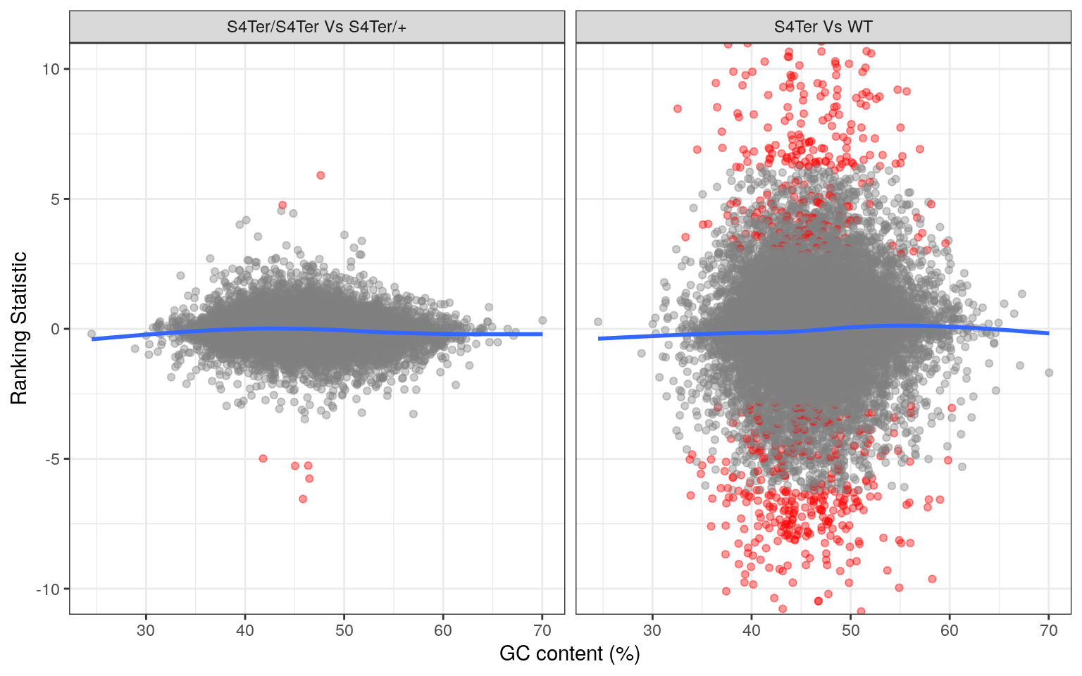
Checks for GC bias in differential expression. GC content is shown against the ranking statistic, using -log10(p) multiplied by the sign of log fold-change. A small amount of bias was noted particularly in the comparison between mutants and wild-type.
topTables %>%
  bind_rows() %>%
  mutate(stat = -sign(logFC)*log10(PValue)) %>%
  ggplot(aes(length, stat)) +
  geom_point(aes(colour = DE), alpha = 0.4) +
  geom_smooth(se = FALSE) +
  facet_wrap(~coef, labeller = contLabeller)  +
  labs(
    x = "Gene Length (bp)",
    y = "Ranking Statistic"
  ) +
  coord_cartesian(ylim = c(-10, 10)) +
  scale_x_log10(labels = comma) +
  scale_colour_manual(values = deCols) +
  theme(legend.position = "none")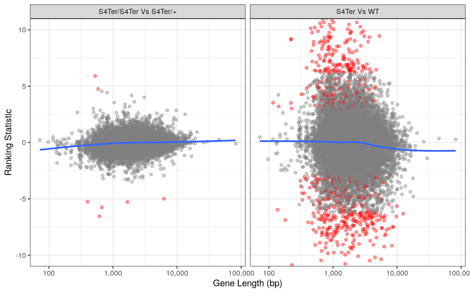
Checks for length bias in differential expression. Gene length is shown against the ranking statistic, using -log10(p) multiplied by the sign of log fold-change. Again, a small amount of bias was noted particularly in the comparison between mutants and wild-type.
Checks for both GC and length bias on differential expression showed that a small bias remained evident, despite using conditional-quantile normalisation. However, an alternative analysis on the same dataset excluding the CQN steps revealed vastly different and exaggerated bias. As such, the impact of CQN normalisation was considered to be appropriate.
Other Artefacts
topTables %>%
  bind_rows() %>%
  arrange(DE) %>%
  ggplot(aes(logCPM, logFC)) +
  geom_point(aes(colour = DE)) +
  geom_text_repel(
    aes(label = gene_name, colour = DE),
    data = . %>% dplyr::filter(DE & abs(logFC) > 2.1)
  ) +
  geom_text_repel(
    aes(label = gene_name, colour = DE),
    data = . %>% dplyr::filter(FDR < 0.05 & coef == "homozygous")
  ) +
  geom_smooth(se = FALSE) +
  geom_hline(
    yintercept = c(-1, 1)*minLfc,
    linetype = 2,
    colour = "red"
  ) +
  facet_wrap(~coef, nrow = 2, labeller = contLabeller) +
  scale_y_continuous(breaks = seq(-8, 8, by = 2)) +
  scale_colour_manual(values = deCols) +
  theme(legend.position = "none")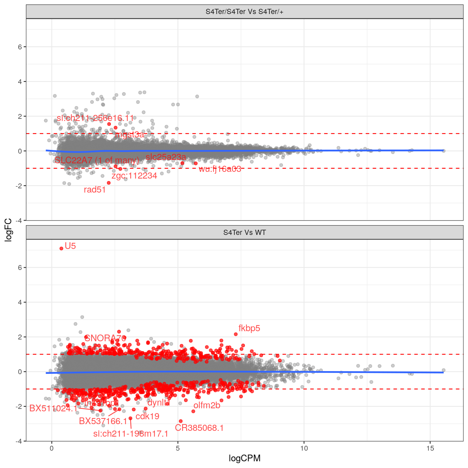
MA plots checking for any logFC bias across the range of expression values. The small curve in the average at the low end of expression values was considered to be an artefact of the sparse points at this end. Initial DE genes are shown in red, with select points labelled.
topTables %>%
  bind_rows() %>%
  ggplot(aes(PValue)) +
  geom_histogram(
    binwidth = 0.02,
    colour = "black", fill = "grey90"
  ) +
  facet_wrap(~coef, labeller = contLabeller)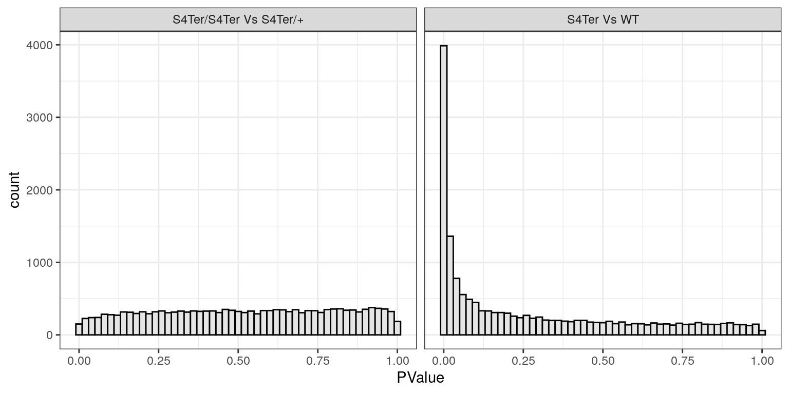
Histograms of p-values for both sets of coefficients. Values for the difference between mutants follow the expected distribution for when there are very few differences, whilst values for the presence of a mutant allele show the expected distribution for when there are many differences. In particular the spike near zero indicates many genes which are differentially expressed.
Results
topTables %>%
  bind_rows() %>%
  ggplot(aes(logFC, -log10(PValue), colour = DE)) +
  geom_point(alpha = 0.4) +
  geom_text_repel(
    aes(label = gene_name),
    data = . %>% dplyr::filter(PValue < 1e-13 | abs(logFC) > 4)
  ) +
  geom_text_repel(
    aes(label = gene_name),
    data = . %>% dplyr::filter(FDR < 0.05 & coef == "homozygous")
  ) +
  geom_vline(
    xintercept = c(-1, 1)*minLfc,
    linetype = 2,
    colour = "red"
  ) +
  facet_wrap(~coef, nrow = 1, labeller = contLabeller) +
  scale_colour_manual(values = deCols) +
  scale_x_continuous(breaks = seq(-8, 8, by = 2)) +
theme(legend.position = "none") 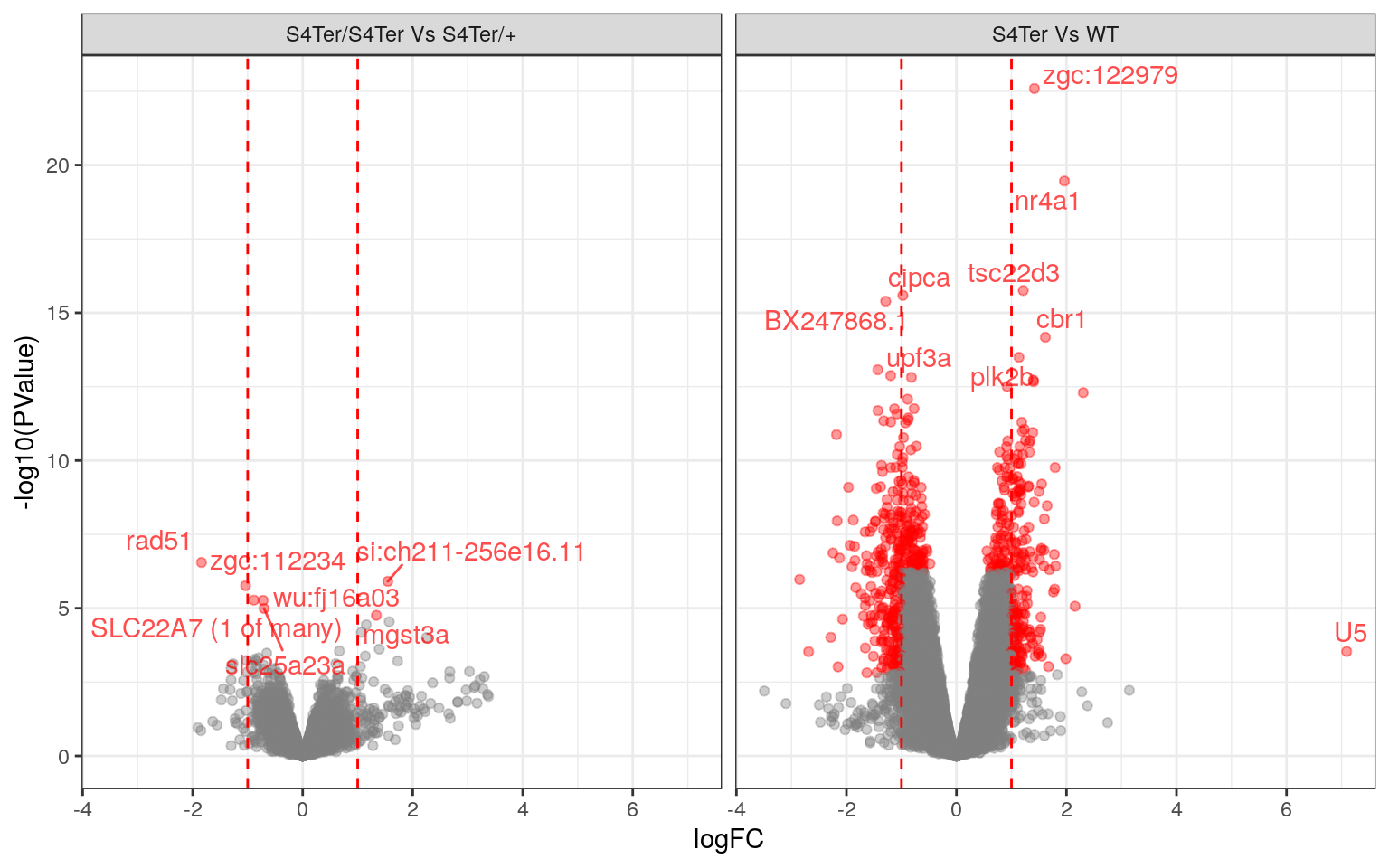
Volcano Plots showing DE genes against logFC.
deGenes <- topTables %>%
  lapply(dplyr::filter, DE) %>%
  lapply(magrittr::extract2, "gene_id")
Genes Tracking with psen2S4Ter
n <- 40A set of 599 genes was identified as DE in the presence of the mutant psen2S4Ter transcript. The most highly ranked 40 genes are shown in the following heatmap. The presence of SNORNA70 in this list is of some concern as this is an ncRNA which is known to interact with ribosomes. In particular the expression pattern follows very closely the patterns previosuly identified for rRNA depletion using the percentage of libraries with GC > 70. For example, WT_86 was the sample with most complete rRNA depletion whilst, Het_84 showed the largest proportion of the library as being derived from rRNA. These represent the samples with lowest and highest expression of SNORNA70 respectively.
genoCols <- RColorBrewer::brewer.pal(3, "Set1") %>%
  setNames(levels(dgeList$samples$genotype))
cpmPostNorm %>%
  extract(deGenes$mutant[seq_len(n)],) %>%
  as.data.frame() %>%
  set_rownames(unlist(geneLabeller(rownames(.)))) %>%
  pheatmap::pheatmap(
    color = viridis_pal(option = "magma")(100),
    labels_col = colnames(.) %>%
      str_replace_all(".+(Het|Hom|WT).+F3(_[0-9]{2}).+", "\\1\\2"),
    legend_breaks = c(seq(-2, 8, by = 2), max(.)),
    legend_labels = c(seq(-2, 8, by = 2), "logCPM\n"),
    annotation_col = dgeList$samples %>%
      dplyr::select(Genotype = genotype),
    annotation_names_col = FALSE,
    annotation_colors = list(Genotype = genoCols),
    cutree_cols = 2,
    cutree_rows = 4
  )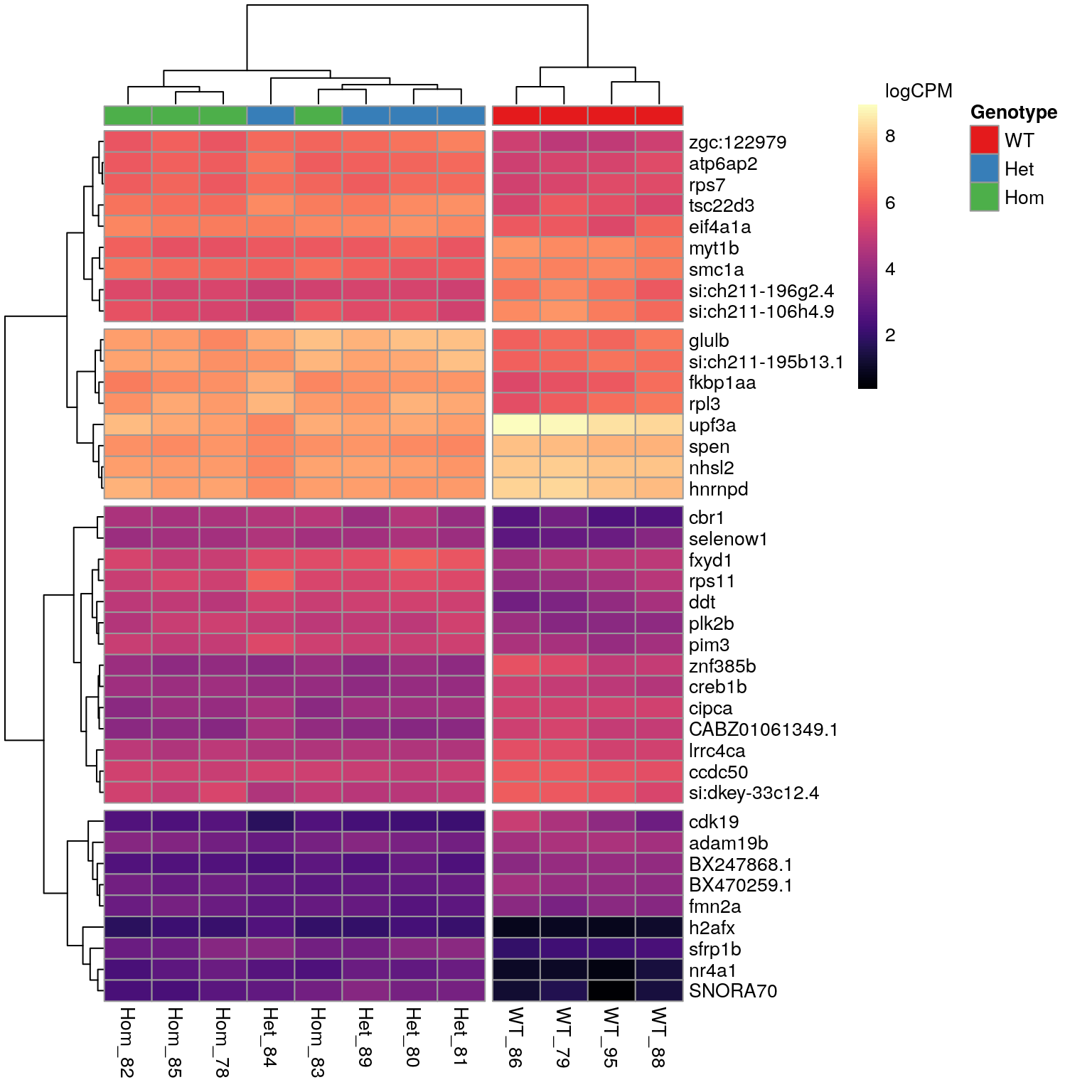
The 40 most highly-ranked genes by FDR which are commonly considered DE between mutants and WT samples. Plotted values are logCPM based on normalised counts.
Genes showing differences between mutants
When inspecting the genes showing differences between mutants, it was noted that the WT and Homozygous mutant samples clustered together, implying that there was a unique effect on these genes which was specific to the heterozygous condition.
cpmPostNorm %>%
  extract(deGenes$homozygous,) %>%
  as.data.frame() %>%
  set_rownames(unlist(geneLabeller(rownames(.)))) %>%
  pheatmap::pheatmap(
    color = viridis_pal(option = "magma")(100),
    labels_col = colnames(.) %>%
      str_replace_all(".+(Het|Hom|WT).+F3(_[0-9]{2}).+", "\\1\\2"),
    legend_breaks = c(seq(-2, 8, by = 2), max(.)),
    legend_labels = c(seq(-2, 8, by = 2), "logCPM\n"),
    annotation_col = dgeList$samples %>%
      dplyr::select(Genotype = genotype),
    annotation_names_col = FALSE,
    annotation_colors = list(Genotype = genoCols),
    cutree_cols = 2,
    cutree_rows = 3
  )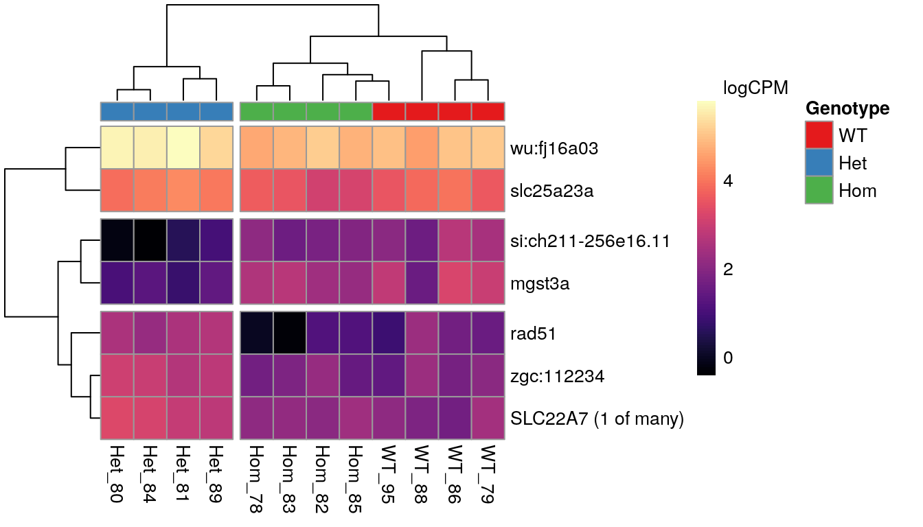
The 7 most highly-ranked genes by FDR which are DE between between mutants. Plotted values are logCPM based on normalised counts.
Data Export
Final gene lists were exported as separate csv files, along with fit and dgeList objects.
write_csv(
  x = topTables$mutant,
  path = here::here("output/psen2VsWT.csv")
)
write_csv(
  x = topTables$homozygous,
  path = here::here("output/psen2HomVsHet.csv")
)
write_rds(
  x = fit,
  path = here::here("data/fit.rds"),
  compress = "gz"
)
write_rds(
  x = dgeList,
  path = here::here("data/dgeList.rds"),
  compress = "gz"
)
write_rds(
  x = cpmPostNorm,
  path = here::here("data/cpmPostNorm.rds"),
  compress = "gz"
)
devtools::session_info()─ Session info ───────────────────────────────────────────────────────────────
setting value
version R version 3.6.3 (2020-02-29)
os Ubuntu 18.04.4 LTS
system x86_64, linux-gnu
ui X11
language en_AU:en
collate en_AU.UTF-8
ctype en_AU.UTF-8
tz Australia/Adelaide
date 2020-04-02
─ Packages ───────────────────────────────────────────────────────────────────
package * version date lib source
AnnotationDbi * 1.48.0 2019-10-29 [2] Bioconductor
AnnotationFilter * 1.10.0 2019-10-29 [2] Bioconductor
AnnotationHub * 2.18.0 2019-10-29 [2] Bioconductor
askpass 1.1 2019-01-13 [2] CRAN (R 3.6.0)
assertthat 0.2.1 2019-03-21 [2] CRAN (R 3.6.0)
backports 1.1.5 2019-10-02 [2] CRAN (R 3.6.1)
Biobase * 2.46.0 2019-10-29 [2] Bioconductor
BiocFileCache * 1.10.2 2019-11-08 [2] Bioconductor
BiocGenerics * 0.32.0 2019-10-29 [2] Bioconductor
BiocManager 1.30.10 2019-11-16 [2] CRAN (R 3.6.1)
BiocParallel 1.20.1 2019-12-21 [2] Bioconductor
BiocVersion 3.10.1 2019-06-06 [2] Bioconductor
biomaRt 2.42.0 2019-10-29 [2] Bioconductor
Biostrings 2.54.0 2019-10-29 [2] Bioconductor
bit 1.1-15.2 2020-02-10 [2] CRAN (R 3.6.2)
bit64 0.9-7 2017-05-08 [2] CRAN (R 3.6.0)
bitops 1.0-6 2013-08-17 [2] CRAN (R 3.6.0)
blob 1.2.1 2020-01-20 [2] CRAN (R 3.6.2)
broom 0.5.4 2020-01-27 [2] CRAN (R 3.6.2)
callr 3.4.2 2020-02-12 [2] CRAN (R 3.6.2)
cellranger 1.1.0 2016-07-27 [2] CRAN (R 3.6.0)
cli 2.0.1 2020-01-08 [2] CRAN (R 3.6.2)
cluster 2.1.0 2019-06-19 [2] CRAN (R 3.6.1)
colorspace 1.4-1 2019-03-18 [2] CRAN (R 3.6.0)
cqn * 1.32.0 2019-10-29 [2] Bioconductor
crayon 1.3.4 2017-09-16 [2] CRAN (R 3.6.0)
curl 4.3 2019-12-02 [2] CRAN (R 3.6.2)
data.table 1.12.8 2019-12-09 [2] CRAN (R 3.6.2)
DBI 1.1.0 2019-12-15 [2] CRAN (R 3.6.2)
dbplyr * 1.4.2 2019-06-17 [2] CRAN (R 3.6.0)
DelayedArray 0.12.2 2020-01-06 [2] Bioconductor
desc 1.2.0 2018-05-01 [2] CRAN (R 3.6.0)
devtools 2.2.2 2020-02-17 [2] CRAN (R 3.6.2)
digest 0.6.25 2020-02-23 [2] CRAN (R 3.6.2)
dplyr * 0.8.4 2020-01-31 [2] CRAN (R 3.6.2)
edgeR * 3.28.1 2020-02-26 [2] Bioconductor
ellipsis 0.3.0 2019-09-20 [2] CRAN (R 3.6.1)
ensembldb * 2.10.2 2019-11-20 [2] Bioconductor
evaluate 0.14 2019-05-28 [2] CRAN (R 3.6.0)
FactoMineR 2.2 2020-02-05 [2] CRAN (R 3.6.2)
fansi 0.4.1 2020-01-08 [2] CRAN (R 3.6.2)
farver 2.0.3 2020-01-16 [2] CRAN (R 3.6.2)
fastmap 1.0.1 2019-10-08 [2] CRAN (R 3.6.1)
flashClust 1.01-2 2012-08-21 [2] CRAN (R 3.6.1)
forcats * 0.4.0 2019-02-17 [2] CRAN (R 3.6.0)
fs 1.3.1 2019-05-06 [2] CRAN (R 3.6.0)
generics 0.0.2 2018-11-29 [2] CRAN (R 3.6.0)
GenomeInfoDb * 1.22.0 2019-10-29 [2] Bioconductor
GenomeInfoDbData 1.2.2 2019-11-21 [2] Bioconductor
GenomicAlignments 1.22.1 2019-11-12 [2] Bioconductor
GenomicFeatures * 1.38.2 2020-02-15 [2] Bioconductor
GenomicRanges * 1.38.0 2019-10-29 [2] Bioconductor
ggdendro 0.1-20 2016-04-27 [2] CRAN (R 3.6.0)
ggplot2 * 3.2.1 2019-08-10 [2] CRAN (R 3.6.1)
ggrepel * 0.8.1 2019-05-07 [2] CRAN (R 3.6.0)
git2r 0.26.1 2019-06-29 [2] CRAN (R 3.6.1)
glue 1.3.1 2019-03-12 [2] CRAN (R 3.6.0)
gtable 0.3.0 2019-03-25 [2] CRAN (R 3.6.0)
haven 2.2.0 2019-11-08 [2] CRAN (R 3.6.1)
here 0.1 2017-05-28 [2] CRAN (R 3.6.0)
highr 0.8 2019-03-20 [2] CRAN (R 3.6.0)
hms 0.5.3 2020-01-08 [2] CRAN (R 3.6.2)
htmltools 0.4.0 2019-10-04 [2] CRAN (R 3.6.1)
htmlwidgets 1.5.1 2019-10-08 [2] CRAN (R 3.6.1)
httpuv 1.5.2 2019-09-11 [2] CRAN (R 3.6.1)
httr 1.4.1 2019-08-05 [2] CRAN (R 3.6.1)
hwriter 1.3.2 2014-09-10 [2] CRAN (R 3.6.0)
interactiveDisplayBase 1.24.0 2019-10-29 [2] Bioconductor
IRanges * 2.20.2 2020-01-13 [2] Bioconductor
jpeg 0.1-8.1 2019-10-24 [2] CRAN (R 3.6.1)
jsonlite 1.6.1 2020-02-02 [2] CRAN (R 3.6.2)
kableExtra 1.1.0 2019-03-16 [2] CRAN (R 3.6.1)
knitr 1.28 2020-02-06 [2] CRAN (R 3.6.2)
labeling 0.3 2014-08-23 [2] CRAN (R 3.6.0)
later 1.0.0 2019-10-04 [2] CRAN (R 3.6.1)
lattice 0.20-40 2020-02-19 [4] CRAN (R 3.6.2)
latticeExtra 0.6-29 2019-12-19 [2] CRAN (R 3.6.2)
lazyeval 0.2.2 2019-03-15 [2] CRAN (R 3.6.0)
leaps 3.1 2020-01-16 [2] CRAN (R 3.6.2)
lifecycle 0.1.0 2019-08-01 [2] CRAN (R 3.6.1)
limma * 3.42.2 2020-02-03 [2] Bioconductor
locfit 1.5-9.1 2013-04-20 [2] CRAN (R 3.6.0)
lubridate 1.7.4 2018-04-11 [2] CRAN (R 3.6.0)
magrittr * 1.5 2014-11-22 [2] CRAN (R 3.6.0)
MASS 7.3-51.5 2019-12-20 [4] CRAN (R 3.6.2)
Matrix 1.2-18 2019-11-27 [2] CRAN (R 3.6.1)
MatrixModels 0.4-1 2015-08-22 [2] CRAN (R 3.6.1)
matrixStats 0.55.0 2019-09-07 [2] CRAN (R 3.6.1)
mclust * 5.4.5 2019-07-08 [2] CRAN (R 3.6.1)
memoise 1.1.0 2017-04-21 [2] CRAN (R 3.6.0)
mgcv 1.8-31 2019-11-09 [4] CRAN (R 3.6.1)
mime 0.9 2020-02-04 [2] CRAN (R 3.6.2)
modelr 0.1.6 2020-02-22 [2] CRAN (R 3.6.2)
munsell 0.5.0 2018-06-12 [2] CRAN (R 3.6.0)
ngsReports * 1.1.2 2019-10-16 [1] Bioconductor
nlme 3.1-144 2020-02-06 [4] CRAN (R 3.6.2)
nor1mix * 1.3-0 2019-06-13 [2] CRAN (R 3.6.1)
openssl 1.4.1 2019-07-18 [2] CRAN (R 3.6.1)
pander * 0.6.3 2018-11-06 [2] CRAN (R 3.6.0)
pheatmap * 1.0.12 2019-01-04 [2] CRAN (R 3.6.0)
pillar 1.4.3 2019-12-20 [2] CRAN (R 3.6.2)
pkgbuild 1.0.6 2019-10-09 [2] CRAN (R 3.6.1)
pkgconfig 2.0.3 2019-09-22 [2] CRAN (R 3.6.1)
pkgload 1.0.2 2018-10-29 [2] CRAN (R 3.6.0)
plotly 4.9.2 2020-02-12 [2] CRAN (R 3.6.2)
plyr 1.8.5 2019-12-10 [2] CRAN (R 3.6.2)
png 0.1-7 2013-12-03 [2] CRAN (R 3.6.0)
preprocessCore * 1.48.0 2019-10-29 [2] Bioconductor
prettyunits 1.1.1 2020-01-24 [2] CRAN (R 3.6.2)
processx 3.4.2 2020-02-09 [2] CRAN (R 3.6.2)
progress 1.2.2 2019-05-16 [2] CRAN (R 3.6.0)
promises 1.1.0 2019-10-04 [2] CRAN (R 3.6.1)
ProtGenerics 1.18.0 2019-10-29 [2] Bioconductor
ps 1.3.2 2020-02-13 [2] CRAN (R 3.6.2)
purrr * 0.3.3 2019-10-18 [2] CRAN (R 3.6.1)
quantreg * 5.54 2019-12-13 [2] CRAN (R 3.6.2)
R6 2.4.1 2019-11-12 [2] CRAN (R 3.6.1)
rappdirs 0.3.1 2016-03-28 [2] CRAN (R 3.6.0)
RColorBrewer * 1.1-2 2014-12-07 [2] CRAN (R 3.6.0)
Rcpp 1.0.3 2019-11-08 [2] CRAN (R 3.6.1)
RCurl 1.98-1.1 2020-01-19 [2] CRAN (R 3.6.2)
readr * 1.3.1 2018-12-21 [2] CRAN (R 3.6.0)
readxl 1.3.1 2019-03-13 [2] CRAN (R 3.6.0)
remotes 2.1.1 2020-02-15 [2] CRAN (R 3.6.2)
reprex 0.3.0 2019-05-16 [2] CRAN (R 3.6.0)
reshape2 1.4.3 2017-12-11 [2] CRAN (R 3.6.0)
rlang 0.4.4 2020-01-28 [2] CRAN (R 3.6.2)
rmarkdown 2.1 2020-01-20 [2] CRAN (R 3.6.2)
rprojroot 1.3-2 2018-01-03 [2] CRAN (R 3.6.0)
Rsamtools 2.2.3 2020-02-23 [2] Bioconductor
RSQLite 2.2.0 2020-01-07 [2] CRAN (R 3.6.2)
rstudioapi 0.11 2020-02-07 [2] CRAN (R 3.6.2)
rtracklayer 1.46.0 2019-10-29 [2] Bioconductor
rvest 0.3.5 2019-11-08 [2] CRAN (R 3.6.1)
S4Vectors * 0.24.3 2020-01-18 [2] Bioconductor
scales * 1.1.0 2019-11-18 [2] CRAN (R 3.6.1)
scatterplot3d 0.3-41 2018-03-14 [2] CRAN (R 3.6.1)
sessioninfo 1.1.1 2018-11-05 [2] CRAN (R 3.6.0)
shiny 1.4.0 2019-10-10 [2] CRAN (R 3.6.1)
ShortRead 1.44.3 2020-02-03 [2] Bioconductor
SparseM * 1.78 2019-12-13 [2] CRAN (R 3.6.2)
stringi 1.4.6 2020-02-17 [2] CRAN (R 3.6.2)
stringr * 1.4.0 2019-02-10 [2] CRAN (R 3.6.0)
SummarizedExperiment 1.16.1 2019-12-19 [2] Bioconductor
testthat 2.3.1 2019-12-01 [2] CRAN (R 3.6.1)
tibble * 2.1.3 2019-06-06 [2] CRAN (R 3.6.0)
tidyr * 1.0.2 2020-01-24 [2] CRAN (R 3.6.2)
tidyselect 1.0.0 2020-01-27 [2] CRAN (R 3.6.2)
tidyverse * 1.3.0 2019-11-21 [2] CRAN (R 3.6.1)
truncnorm 1.0-8 2018-02-27 [2] CRAN (R 3.6.0)
usethis 1.5.1 2019-07-04 [2] CRAN (R 3.6.1)
vctrs 0.2.3 2020-02-20 [2] CRAN (R 3.6.2)
viridisLite 0.3.0 2018-02-01 [2] CRAN (R 3.6.0)
webshot 0.5.2 2019-11-22 [2] CRAN (R 3.6.1)
whisker 0.4 2019-08-28 [2] CRAN (R 3.6.1)
withr 2.1.2 2018-03-15 [2] CRAN (R 3.6.0)
workflowr * 1.6.0 2019-12-19 [2] CRAN (R 3.6.2)
xfun 0.12 2020-01-13 [2] CRAN (R 3.6.2)
XML 3.99-0.3 2020-01-20 [2] CRAN (R 3.6.2)
xml2 1.2.2 2019-08-09 [2] CRAN (R 3.6.1)
xtable 1.8-4 2019-04-21 [2] CRAN (R 3.6.0)
XVector 0.26.0 2019-10-29 [2] Bioconductor
yaml 2.2.1 2020-02-01 [2] CRAN (R 3.6.2)
zlibbioc 1.32.0 2019-10-29 [2] Bioconductor
zoo 1.8-7 2020-01-10 [2] CRAN (R 3.6.2)
[1] /home/steveped/R/x86_64-pc-linux-gnu-library/3.6
[2] /usr/local/lib/R/site-library
[3] /usr/lib/R/site-library
[4] /usr/lib/R/library