Analysis Without Using CQN
Steve Pederson
2020-01-24
Last updated: 2020-04-02
Checks: 7 0
Knit directory: 20170327_Psen2S4Ter_RNASeq/
This reproducible R Markdown analysis was created with workflowr (version 1.6.0). The Checks tab describes the reproducibility checks that were applied when the results were created. The Past versions tab lists the development history.
Great! Since the R Markdown file has been committed to the Git repository, you know the exact version of the code that produced these results.
Great job! The global environment was empty. Objects defined in the global environment can affect the analysis in your R Markdown file in unknown ways. For reproduciblity it’s best to always run the code in an empty environment.
The command set.seed(20200119) was run prior to running the code in the R Markdown file. Setting a seed ensures that any results that rely on randomness, e.g. subsampling or permutations, are reproducible.
Great job! Recording the operating system, R version, and package versions is critical for reproducibility.
Nice! There were no cached chunks for this analysis, so you can be confident that you successfully produced the results during this run.
Great job! Using relative paths to the files within your workflowr project makes it easier to run your code on other machines.
Great! You are using Git for version control. Tracking code development and connecting the code version to the results is critical for reproducibility. The version displayed above was the version of the Git repository at the time these results were generated.
Note that you need to be careful to ensure that all relevant files for the analysis have been committed to Git prior to generating the results (you can use wflow_publish or wflow_git_commit). workflowr only checks the R Markdown file, but you know if there are other scripts or data files that it depends on. Below is the status of the Git repository when the results were generated:
Ignored files:
    Ignored:    .Rhistory
    Ignored:    .Rproj.user/

Untracked files:
    Untracked:  basic_sample_checklist.txt
    Untracked:  experiment_paired_fastq_spreadsheet_template.txt

Unstaged changes:
    Modified:   analysis/_site.yml
    Modified:   data/cpmPostNorm.rds
    Modified:   data/dgeList.rds
    Modified:   data/fit.rds
    Modified:   output/psen2HomVsHet.csv
    Modified:   output/psen2VsWT.csv

Staged changes:
    Modified:   analysis/_site.yml
Note that any generated files, e.g. HTML, png, CSS, etc., are not included in this status report because it is ok for generated content to have uncommitted changes.
These are the previous versions of the R Markdown and HTML files. If you’ve configured a remote Git repository (see ?wflow_git_remote), click on the hyperlinks in the table below to view them.
| File | Version | Author | Date | Message |
|---|---|---|---|---|
| html | 876e40f | Steve Ped | 2020-02-17 | Compiled after minor corrections |
| html | 96d8cc7 | Steve Ped | 2020-01-25 | Compiled after data export & added compression to output |
| Rmd | be95a60 | Steve Ped | 2020-01-25 | Finished first pass of DE Analysis |
| html | be95a60 | Steve Ped | 2020-01-25 | Finished first pass of DE Analysis |
| html | 9bff516 | Steve Ped | 2020-01-24 | Added analysis without CQN |
| Rmd | 7b680b2 | Steve Ped | 2020-01-24 | Added analysis without CQN |
Introduction
This workflow is an alternative differential gene expression analysis, however conditional quantile normalisation was not used. This was written up specifically to allow for a checking of the impact this method has had on the dataset.
library(ngsReports)
library(tidyverse)
library(magrittr)
library(edgeR)
library(AnnotationHub)
library(ensembldb)
library(scales)
library(pander)
library(cowplot)
library(cqn)
library(ggrepel)
library(UpSetR)
if (interactive()) setwd(here::here())
theme_set(theme_bw())
panderOptions("big.mark", ",")
panderOptions("table.split.table", Inf)
panderOptions("table.style", "rmarkdown")
twoCols <- c(rgb(0.8, 0.1, 0.1), rgb(0.2, 0.2, 0.8))Annotations
ah <- AnnotationHub() %>%
    subset(species == "Danio rerio") %>%
    subset(rdataclass == "EnsDb")
ensDb <- ah[["AH74989"]]
grTrans <- transcripts(ensDb)
trLengths <- exonsBy(ensDb, "tx") %>%
width() %>%
vapply(sum, integer(1))
mcols(grTrans)$length <- trLengths[names(grTrans)]gcGene <- grTrans %>%
mcols() %>%
as.data.frame() %>%
dplyr::select(gene_id, tx_id, gc_content, length) %>%
as_tibble() %>%
group_by(gene_id) %>%
summarise(
gc_content = sum(gc_content*length) / sum(length),
length = ceiling(median(length))
)
grGenes <- genes(ensDb)
mcols(grGenes) %<>%
as.data.frame() %>%
left_join(gcGene) %>%
as.data.frame() %>%
DataFrame()Similarly to the Quality Assessment steps, GRanges objects were formed at the gene and transcript levels, to enable estimation of GC content and length for each transcript and gene. GC content and transcript length are available for each transcript, and for gene-level estimates, GC content was taken as the sum of all GC bases divided by the sum of all transcript lengths, effectively averaging across all transcripts. Gene length was defined as the median transcript length.
samples <- read_csv("data/samples.csv") %>%
    distinct(sampleName, .keep_all = TRUE) %>%
    dplyr::select(sample = sampleName, sampleID, genotype) %>%
    mutate(genotype = factor(genotype, levels = c("WT", "Het", "Hom")))
Sample metadata was also loaded, with only the sampleID and genotype being retained. All other fields were considered irrelevant.
Count Data
minCPM <- 1.5
minSamples <- 4
dgeList <- file.path("data", "2_alignedData", "featureCounts", "genes.out") %>%
    read_delim(delim = "\t") %>%
    set_names(basename(names(.))) %>%
    as.data.frame() %>%
    column_to_rownames("Geneid") %>%
    as.matrix() %>%
    set_colnames(str_remove(colnames(.), "Aligned.sortedByCoord.out.bam")) %>%
    .[rowSums(cpm(.) >= minCPM) >= minCPM,] %>%
    DGEList(
        samples = tibble(sample = colnames(.)) %>%
            left_join(samples),
        genes = grGenes[rownames(.)] %>%
            as.data.frame() %>%
            dplyr::select(
                chromosome = seqnames, start, end,
                gene_id, gene_name, gene_biotype, description,
                entrezid, gc_content, length
            )
    ) %>%
    .[!grepl("rRNA", .$genes$gene_biotype),] %>%
    calcNormFactors()
Gene-level count data as output by featureCounts, was loaded and formed into a DGEList object. During this process, genes were removed if:
- They were not considered as detectable (CPM < 1.5 in > 8 samples). This translates to > 18 reads assigned a gene in all samples from one or more of the genotype groups
- The
gene_biotypewas any type ofrRNA.
These filtering steps returned gene-level counts for 16,640 genes, with total library sizes between 11,852,141 and 16,997,219 reads assigned to genes. It was noted that these library sizes were about 1.5-fold larger than the transcript-level counts used for the QA steps.
cpm(dgeList, log = TRUE) %>%
    as.data.frame() %>%
    pivot_longer(
        cols = everything(),
        names_to = "sample",
        values_to = "logCPM"
    ) %>%
    split(f = .$sample) %>%
    lapply(function(x){
        d <- density(x$logCPM)
        tibble(
            sample = unique(x$sample),
            x = d$x,
            y = d$y
        )
    }) %>%
    bind_rows() %>%
    left_join(samples) %>%
    ggplot(aes(x, y, colour = genotype, group = sample)) +
    geom_line() +
    labs(
        x = "logCPM",
        y = "Density",
        colour = "Genotype"
    )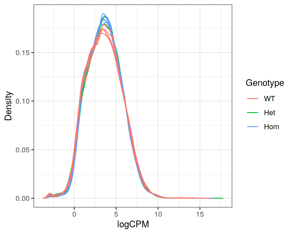
Expression density plots for all samples after filtering, showing logCPM values.
| Version | Author | Date |
|---|---|---|
| 9bff516 | Steve Ped | 2020-01-24 |
Additional Functions
contLabeller <- as_labeller(
    c(
        HetVsWT = "S4Ter/+ Vs +/+",
        HomVsWT = "S4Ter/S4Ter Vs +/+",
        HomVsHet = "S4Ter/S4Ter Vs S4Ter/+",
        Hom = "S4Ter/S4Ter",
        Het = "S4Ter/+",
        WT = "+/+"
    )
)
geneLabeller <- structure(grGenes$gene_name, names = grGenes$gene_id) %>%
    as_labeller()
Labeller functions for genotypes, contrasts and gene names were additionally defined for simpler plotting using ggplot2.
Analysis Using NB Models
Model Description
The same model was applied as for the analysis using CQN.
d <- model.matrix(~ 0 + genotype, data = dgeList$samples) %>%
    set_colnames(str_remove_all(colnames(.), "genotype"))
cont <- makeContrasts(
    HetVsWT = Het - WT,
    HomVsWT = Hom - WT,
    HomVsHet = Hom - Het,
    levels = d
)
Normalisation
No GC normalisation was included in this workflow. Instead, dispersions were calculated using the model matrix as defined in the full workflow.
dgeList %<>% estimateDisp(design = d)Model Fitting
minLfc <- log2(1.5)
alpha <- 0.01
fit <- glmFit(dgeList)
topTables <- colnames(cont) %>%
    sapply(function(x){
        glmLRT(fit, contrast = cont[,x]) %>%
            topTags(n = Inf) %>%
            .[["table"]] %>%
            as_tibble() %>%
            dplyr::select(
                gene_id, gene_name, logFC, logCPM, PValue, FDR, everything()
            ) %>%
            mutate(
                comparison = x,
                DE = FDR < alpha & abs(logFC) > minLfc
            )
    },
    simplify = FALSE)
Models were fit using the negative-binomial approaches of glmFit(). Top Tables were then obtained using pair-wise likelihood-ratio tests in glmLRT(). These test the standard \(H_0\) that there is no difference in gene expression estimates between genotypes, the gene expression estimates are obtained under the negative binomial model.
alpha2 <- 0.05
topTables %<>%
  bind_rows() %>%
  split(f = .$gene_id) %>%
  lapply(function(x){mutate(x, DE = any(DE) & FDR < alpha2)}) %>%
  bind_rows() %>%
  split(f = .$comparison)
In order to remain as comparable as possible, the same secondary gene selection steps were performed as for the main analysis.
For enrichment testing, genes were initially considered to be DE using an estimated logFC outside of the range \(\pm \log_2(1.5)\) and an FDR-adjusted p-value < 0.01. For genes in any of these initial lists, the logFC filter was subsequently removed from subsequent comparisons in order to minimise issues introduced by the use of a hard cutoff. Similarly the FDR threshold was raised to 0.05 in secondary comparisons for genes which passed the initial round of selection.
Using these criteria, the following initial DE gene-sets were defined. These were slightly higher than previously
topTables %>%
  lapply(dplyr::filter, DE) %>%
  vapply(nrow, integer(1)) %>%
pander()| HetVsWT | HomVsHet | HomVsWT |
|---|---|---|
| 2,399 | 7 | 2,043 |
Model Checking
topTables %>%
  bind_rows() %>%
  ggplot(aes(logCPM, logFC)) +
  geom_point(aes(colour = DE), alpha = 0.4) +
  geom_text_repel(
    aes(label = gene_name, colour = DE),
    data = . %>% dplyr::filter(DE & abs(logFC) > 3)
  ) +
  geom_text_repel(
    aes(label = gene_name, colour = DE),
    data = . %>% dplyr::filter(FDR < 0.05 & comparison == "HomVsHet")
  ) +
  geom_smooth(se = FALSE) +
  geom_hline(
    yintercept = c(-1, 1)*minLfc,
    linetype = 2,
    colour = "red"
  ) +
  facet_wrap(~comparison, nrow = 1, labeller = contLabeller) +
  scale_y_continuous(breaks = seq(-8, 8, by = 2)) +
  scale_colour_manual(values = c("grey50", "red")) +
  theme(legend.position = "none")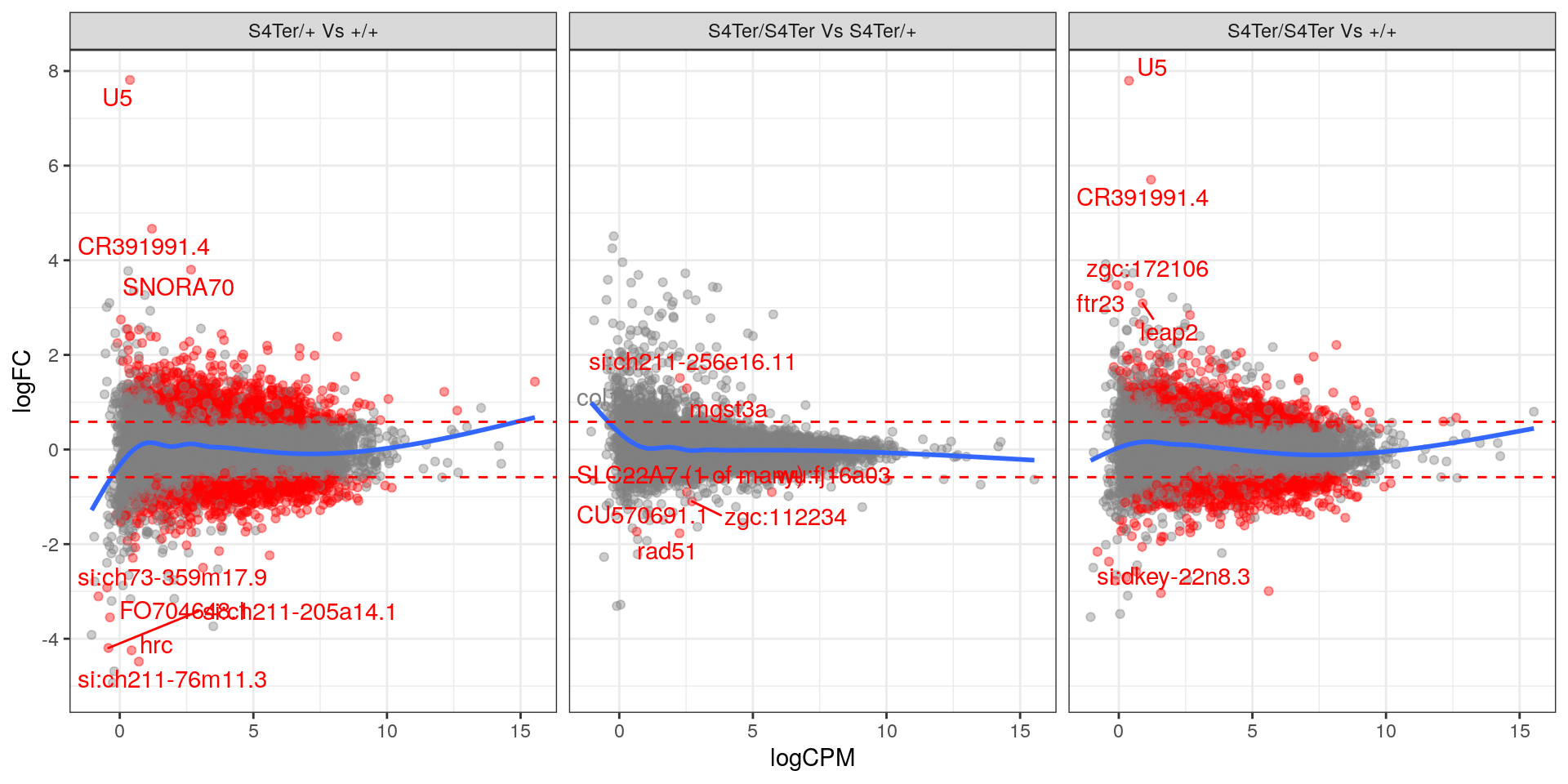
MA plots checking for any logFC bias across the range of expression values. Both mutant comparisons against wild-type appear to show a biased relationship between logFC and expression level.. Initial DE genes are shown in red, with select points labelled.
| Version | Author | Date |
|---|---|---|
| 9bff516 | Steve Ped | 2020-01-24 |
topTables %>%
    bind_rows() %>%
    mutate(stat = -sign(logFC)*log10(PValue)) %>%
    ggplot(aes(gc_content, stat)) +
    geom_point(aes(colour = DE), alpha = 0.4) +
    geom_smooth(se = FALSE) +
    facet_wrap(~comparison, labeller = contLabeller)  +
    labs(
        x = "GC content (%)",
        y = "Ranking Statistic"
    ) +
    coord_cartesian(ylim = c(-10, 10)) +
    scale_colour_manual(values = c("grey50", "red")) +
    theme(legend.position = "none")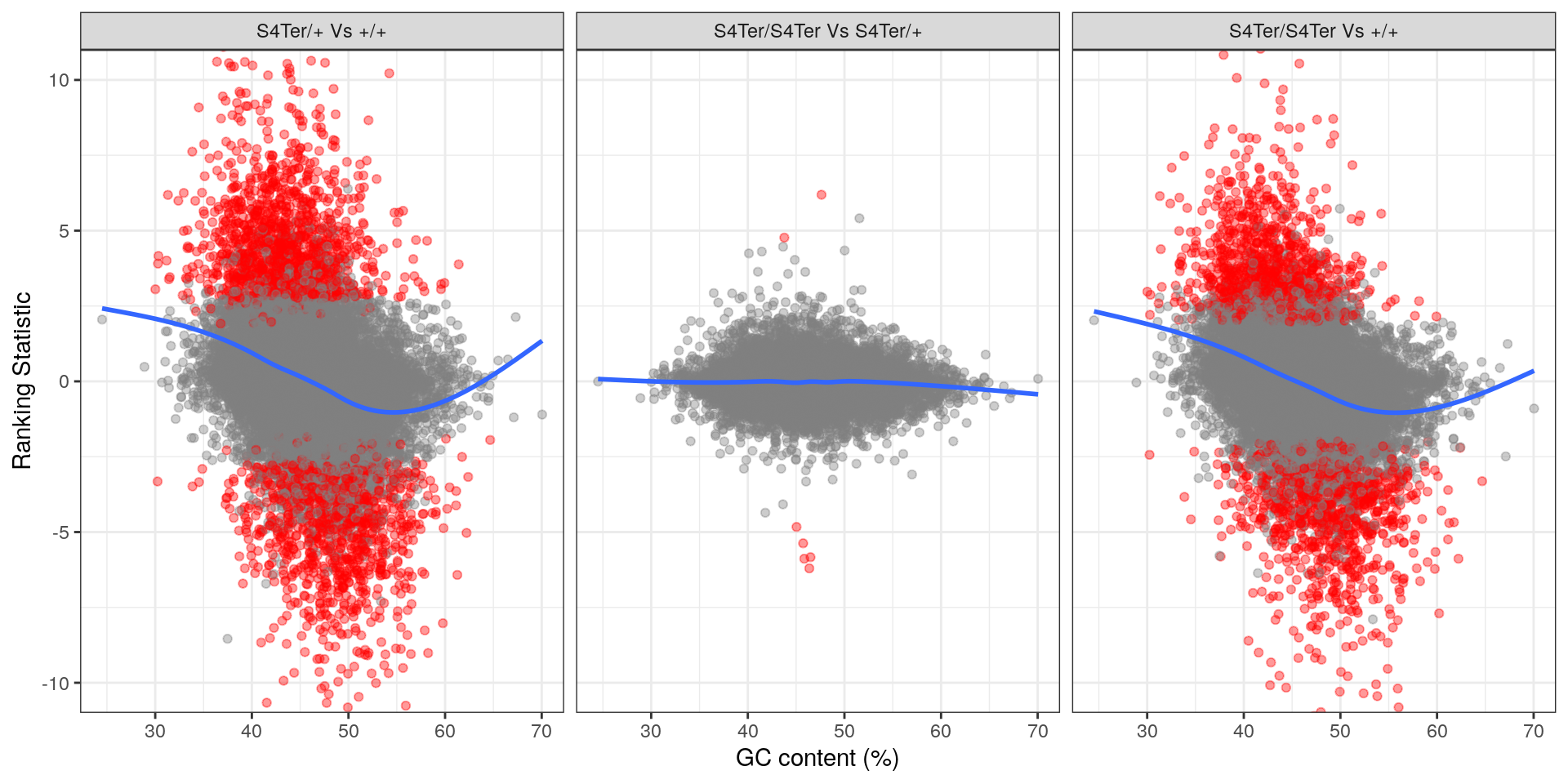
Checks for GC bias in differential expression. GC content is shown against the ranking statistic, using -log10(p) multiplied by the sign of log fold-change. A large amount of bias was noted particularly in the comparison between homozygous mutants and wild-type.
| Version | Author | Date |
|---|---|---|
| 9bff516 | Steve Ped | 2020-01-24 |
topTables %>%
    bind_rows() %>%
    mutate(stat = -sign(logFC)*log10(PValue)) %>%
    ggplot(aes(length, stat)) +
    geom_point(aes(colour = DE), alpha = 0.4) +
    geom_smooth(se = FALSE) +
    facet_wrap(~comparison, labeller = contLabeller)  +
    labs(
        x = "Gene Length (bp)",
        y = "Ranking Statistic"
    ) +
    coord_cartesian(ylim = c(-10, 10)) +
    scale_x_log10(labels = comma) +
    scale_colour_manual(values = c("grey50", "red")) +
    theme(legend.position = "none")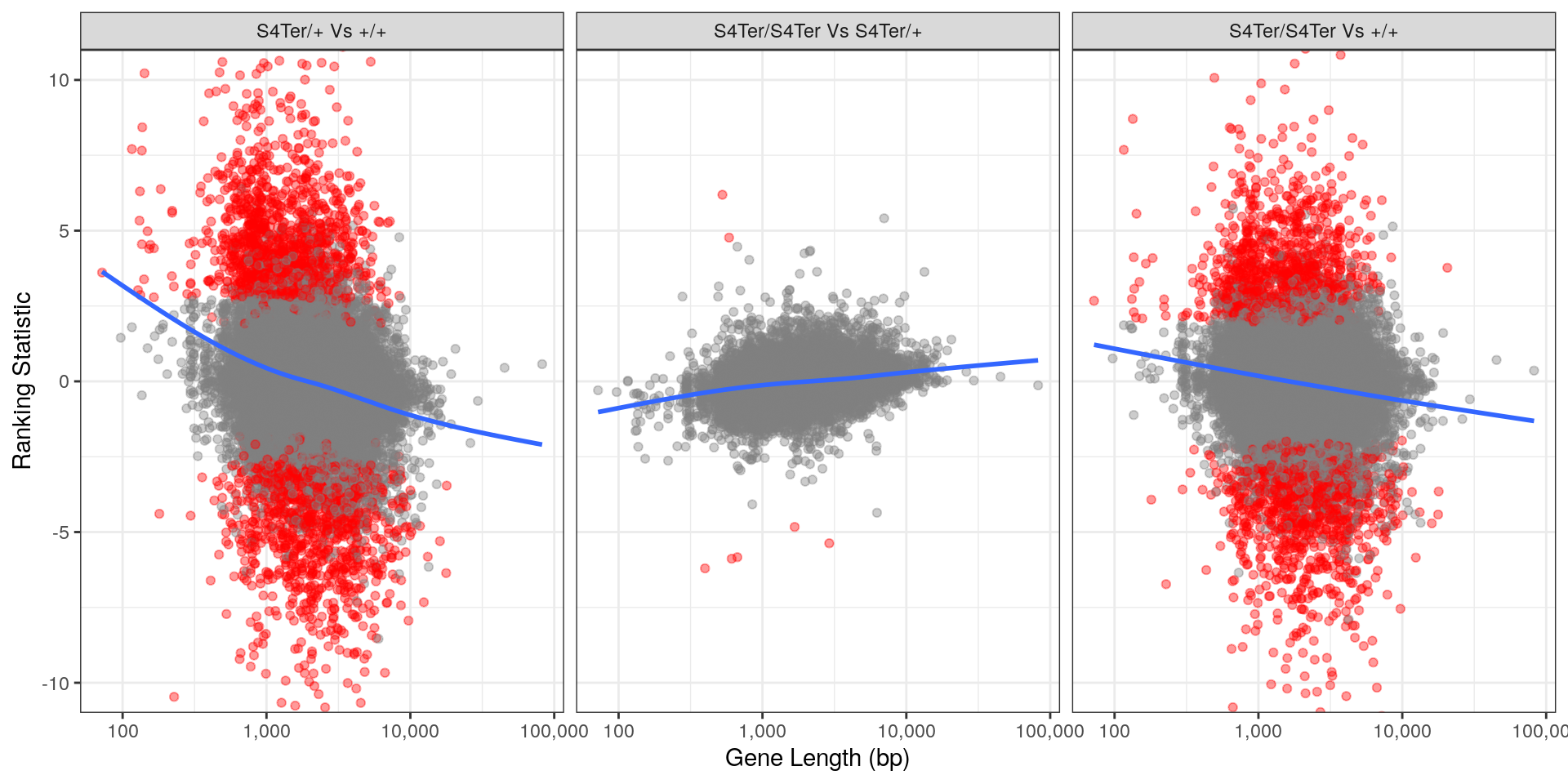
Checks for length bias in differential expression. Gene length is shown against the ranking statistic, using -log10(p) multiplied by the sign of log fold-change. Again, a large amount of bias was noted particularly in the comparison between homozygous mutants and wild-type.
| Version | Author | Date |
|---|---|---|
| 9bff516 | Steve Ped | 2020-01-24 |
Analysis Using Voom
As a final alternative, the dataset was fit using voomWithQualityWeights(). Given that two samples were relatively divergent from the remainder of the samples, in terms of their rRNA depletion, this strategy may resolve some of these issues.
voomData <- dgeList %>%
    voomWithQualityWeights(design = matrix(1, nrow = ncol(.)))
voomFit <- voomData %>%
    lmFit(design = d) %>%
    contrasts.fit(cont) %>%
    eBayes()
voomData$targets %>%
ggplot(aes(sampleID, sample.weights, fill = genotype)) +
geom_bar(stat = "identity") +
facet_wrap(~genotype, labeller = contLabeller, scales = "free_x") +
theme(legend.position = "none")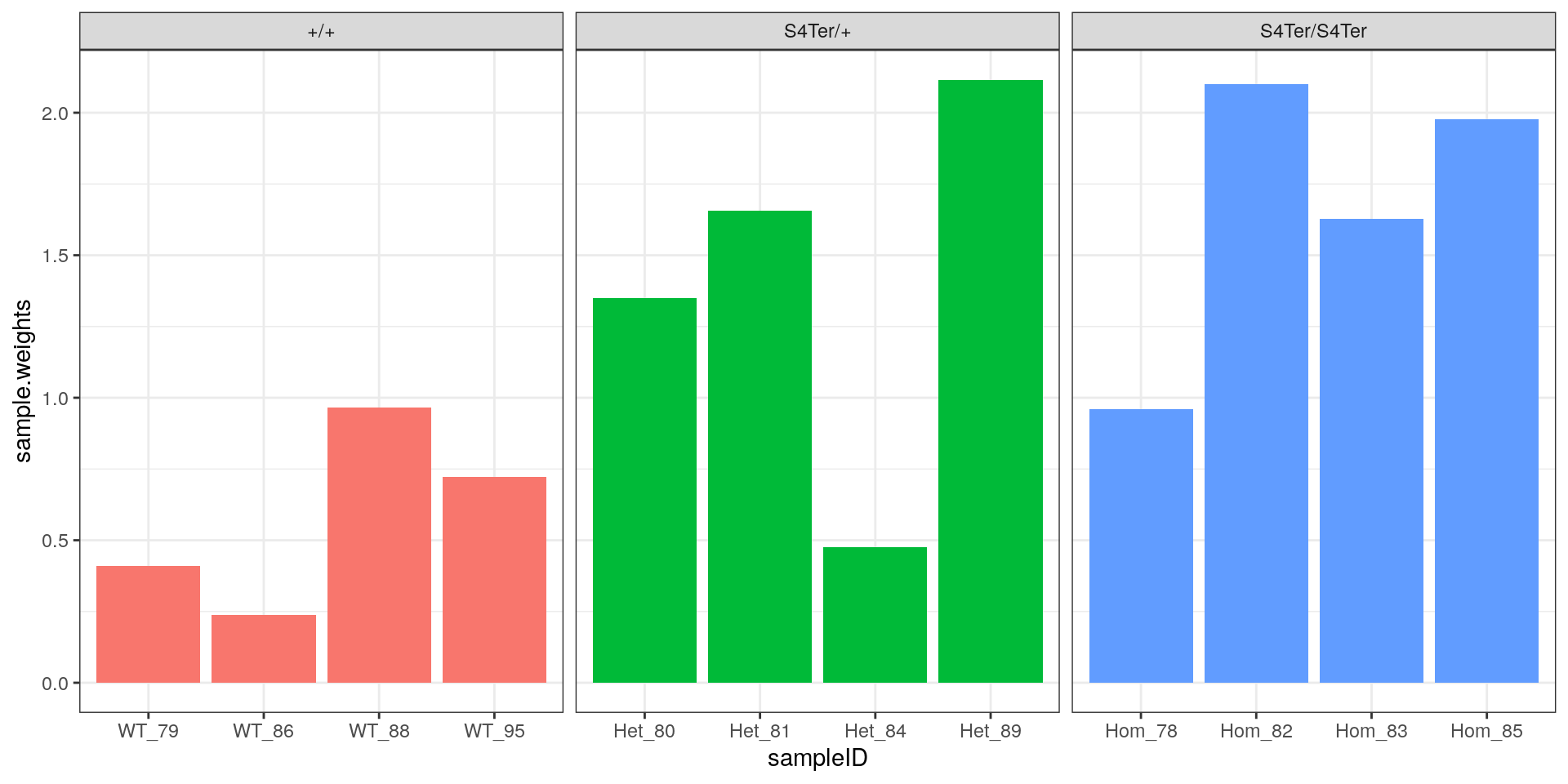
Sample-level weights after applying voom. As expected, the highest and lowest samples from the initial rRNA analysis were down-weighted the most strongly
| Version | Author | Date |
|---|---|---|
| 9bff516 | Steve Ped | 2020-01-24 |
voomTables <- colnames(cont) %>%
    sapply(function(x){
        topTable(voomFit, coef = x, number = Inf) %>%
            as_tibble() %>%
            dplyr::select(
                gene_id, gene_name, logFC, AveExpr, P.Value, FDR = adj.P.Val, everything()
            ) %>%
            mutate(
                comparison = x,
                DE = FDR < alpha & abs(logFC) > minLfc
            )
    },
    simplify = FALSE)
Model Checking
voomTables %>%
  bind_rows() %>%
  ggplot(aes(AveExpr, logFC)) +
  geom_point(aes(colour = DE), alpha = 0.4) +
  geom_text_repel(
    aes(label = gene_name, colour = DE),
    data = . %>% dplyr::filter(DE & abs(logFC) > 3)
  ) +
  geom_text_repel(
    aes(label = gene_name, colour = DE),
    data = . %>% dplyr::filter(FDR < 0.05 & comparison == "HomVsHet")
  ) +
  geom_smooth(se = FALSE) +
  geom_hline(
    yintercept = c(-1, 1)*minLfc,
    linetype = 2,
    colour = "red"
  ) +
  facet_wrap(~comparison, nrow = 1, labeller = contLabeller) +
  scale_y_continuous(breaks = seq(-8, 8, by = 2)) +
  scale_colour_manual(values = c("grey50", "red")) +
  theme(legend.position = "none")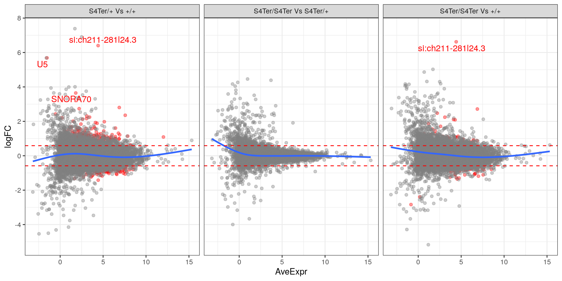
MA plots checking for any logFC bias across the range of expression values. Both mutant comparisons against wild-type appear to show a biased relationship between logFC and expression level.. Initial DE genes are shown in red, with select points labelled.
| Version | Author | Date |
|---|---|---|
| 9bff516 | Steve Ped | 2020-01-24 |
voomTables %>%
    bind_rows() %>%
    ggplot(aes(gc_content, t)) +
    geom_point(aes(colour = DE), alpha = 0.4) +
    geom_smooth(se = FALSE) +
    facet_wrap(~comparison, labeller = contLabeller)  +
    labs(
        x = "GC content (%)",
        y = "Ranking Statistic (t)"
    ) +
    coord_cartesian(ylim = c(-10, 10)) +
    scale_colour_manual(values = c("grey50", "red")) +
    theme(legend.position = "none")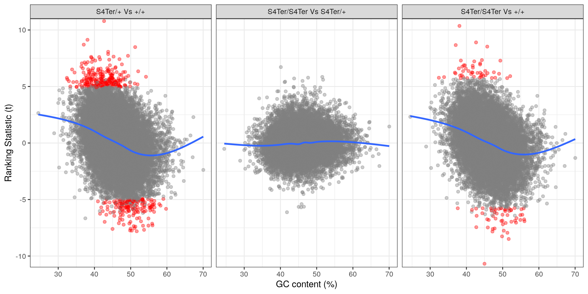
Checks for GC bias in differential expression. GC content is shown against the ranking t-statistic. A large amount of bias was noted particularly in the comparison between homozygous mutants and wild-type.
| Version | Author | Date |
|---|---|---|
| 9bff516 | Steve Ped | 2020-01-24 |
voomTables %>%
    bind_rows() %>%
    ggplot(aes(length, t)) +
    geom_point(aes(colour = DE), alpha = 0.4) +
    geom_smooth(se = FALSE) +
    facet_wrap(~comparison, labeller = contLabeller)  +
    labs(
        x = "Gene Length (bp)",
        y = "Ranking Statistic (t)"
    ) +
    coord_cartesian(ylim = c(-10, 10)) +
    scale_x_log10(labels = comma) +
    scale_colour_manual(values = c("grey50", "red")) +
    theme(legend.position = "none")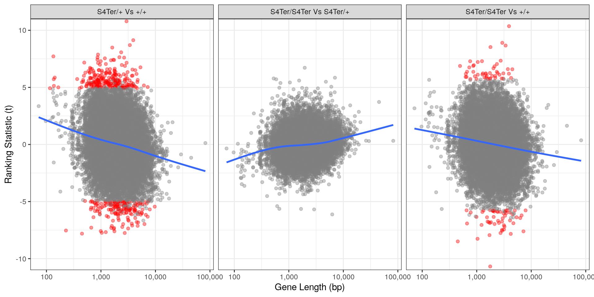
Checks for length bias in differential expression. Gene length is shown against the ranking t-statistic. Again, a large amount of bias was noted particularly in the comparison between homozygous mutants and wild-type.
| Version | Author | Date |
|---|---|---|
| 9bff516 | Steve Ped | 2020-01-24 |
Conclusion
None of the results in this workflow were for analysis, but were simply to assess the impact of GC and length bias without accounting for it using CQN.
devtools::session_info()─ Session info ───────────────────────────────────────────────────────────────
setting value
version R version 3.6.3 (2020-02-29)
os Ubuntu 18.04.4 LTS
system x86_64, linux-gnu
ui X11
language en_AU:en
collate en_AU.UTF-8
ctype en_AU.UTF-8
tz Australia/Adelaide
date 2020-04-02
─ Packages ───────────────────────────────────────────────────────────────────
package * version date lib source
AnnotationDbi * 1.48.0 2019-10-29 [2] Bioconductor
AnnotationFilter * 1.10.0 2019-10-29 [2] Bioconductor
AnnotationHub * 2.18.0 2019-10-29 [2] Bioconductor
askpass 1.1 2019-01-13 [2] CRAN (R 3.6.0)
assertthat 0.2.1 2019-03-21 [2] CRAN (R 3.6.0)
backports 1.1.5 2019-10-02 [2] CRAN (R 3.6.1)
Biobase * 2.46.0 2019-10-29 [2] Bioconductor
BiocFileCache * 1.10.2 2019-11-08 [2] Bioconductor
BiocGenerics * 0.32.0 2019-10-29 [2] Bioconductor
BiocManager 1.30.10 2019-11-16 [2] CRAN (R 3.6.1)
BiocParallel 1.20.1 2019-12-21 [2] Bioconductor
BiocVersion 3.10.1 2019-06-06 [2] Bioconductor
biomaRt 2.42.0 2019-10-29 [2] Bioconductor
Biostrings 2.54.0 2019-10-29 [2] Bioconductor
bit 1.1-15.2 2020-02-10 [2] CRAN (R 3.6.2)
bit64 0.9-7 2017-05-08 [2] CRAN (R 3.6.0)
bitops 1.0-6 2013-08-17 [2] CRAN (R 3.6.0)
blob 1.2.1 2020-01-20 [2] CRAN (R 3.6.2)
broom 0.5.4 2020-01-27 [2] CRAN (R 3.6.2)
callr 3.4.2 2020-02-12 [2] CRAN (R 3.6.2)
cellranger 1.1.0 2016-07-27 [2] CRAN (R 3.6.0)
cli 2.0.1 2020-01-08 [2] CRAN (R 3.6.2)
cluster 2.1.0 2019-06-19 [2] CRAN (R 3.6.1)
colorspace 1.4-1 2019-03-18 [2] CRAN (R 3.6.0)
cowplot * 1.0.0 2019-07-11 [2] CRAN (R 3.6.1)
cqn * 1.32.0 2019-10-29 [2] Bioconductor
crayon 1.3.4 2017-09-16 [2] CRAN (R 3.6.0)
curl 4.3 2019-12-02 [2] CRAN (R 3.6.2)
data.table 1.12.8 2019-12-09 [2] CRAN (R 3.6.2)
DBI 1.1.0 2019-12-15 [2] CRAN (R 3.6.2)
dbplyr * 1.4.2 2019-06-17 [2] CRAN (R 3.6.0)
DelayedArray 0.12.2 2020-01-06 [2] Bioconductor
desc 1.2.0 2018-05-01 [2] CRAN (R 3.6.0)
devtools 2.2.2 2020-02-17 [2] CRAN (R 3.6.2)
digest 0.6.25 2020-02-23 [2] CRAN (R 3.6.2)
dplyr * 0.8.4 2020-01-31 [2] CRAN (R 3.6.2)
edgeR * 3.28.1 2020-02-26 [2] Bioconductor
ellipsis 0.3.0 2019-09-20 [2] CRAN (R 3.6.1)
ensembldb * 2.10.2 2019-11-20 [2] Bioconductor
evaluate 0.14 2019-05-28 [2] CRAN (R 3.6.0)
FactoMineR 2.2 2020-02-05 [2] CRAN (R 3.6.2)
fansi 0.4.1 2020-01-08 [2] CRAN (R 3.6.2)
farver 2.0.3 2020-01-16 [2] CRAN (R 3.6.2)
fastmap 1.0.1 2019-10-08 [2] CRAN (R 3.6.1)
flashClust 1.01-2 2012-08-21 [2] CRAN (R 3.6.1)
forcats * 0.4.0 2019-02-17 [2] CRAN (R 3.6.0)
fs 1.3.1 2019-05-06 [2] CRAN (R 3.6.0)
generics 0.0.2 2018-11-29 [2] CRAN (R 3.6.0)
GenomeInfoDb * 1.22.0 2019-10-29 [2] Bioconductor
GenomeInfoDbData 1.2.2 2019-11-21 [2] Bioconductor
GenomicAlignments 1.22.1 2019-11-12 [2] Bioconductor
GenomicFeatures * 1.38.2 2020-02-15 [2] Bioconductor
GenomicRanges * 1.38.0 2019-10-29 [2] Bioconductor
ggdendro 0.1-20 2016-04-27 [2] CRAN (R 3.6.0)
ggplot2 * 3.2.1 2019-08-10 [2] CRAN (R 3.6.1)
ggrepel * 0.8.1 2019-05-07 [2] CRAN (R 3.6.0)
git2r 0.26.1 2019-06-29 [2] CRAN (R 3.6.1)
glue 1.3.1 2019-03-12 [2] CRAN (R 3.6.0)
gridExtra 2.3 2017-09-09 [2] CRAN (R 3.6.0)
gtable 0.3.0 2019-03-25 [2] CRAN (R 3.6.0)
haven 2.2.0 2019-11-08 [2] CRAN (R 3.6.1)
highr 0.8 2019-03-20 [2] CRAN (R 3.6.0)
hms 0.5.3 2020-01-08 [2] CRAN (R 3.6.2)
htmltools 0.4.0 2019-10-04 [2] CRAN (R 3.6.1)
htmlwidgets 1.5.1 2019-10-08 [2] CRAN (R 3.6.1)
httpuv 1.5.2 2019-09-11 [2] CRAN (R 3.6.1)
httr 1.4.1 2019-08-05 [2] CRAN (R 3.6.1)
hwriter 1.3.2 2014-09-10 [2] CRAN (R 3.6.0)
interactiveDisplayBase 1.24.0 2019-10-29 [2] Bioconductor
IRanges * 2.20.2 2020-01-13 [2] Bioconductor
jpeg 0.1-8.1 2019-10-24 [2] CRAN (R 3.6.1)
jsonlite 1.6.1 2020-02-02 [2] CRAN (R 3.6.2)
kableExtra 1.1.0 2019-03-16 [2] CRAN (R 3.6.1)
knitr 1.28 2020-02-06 [2] CRAN (R 3.6.2)
labeling 0.3 2014-08-23 [2] CRAN (R 3.6.0)
later 1.0.0 2019-10-04 [2] CRAN (R 3.6.1)
lattice 0.20-40 2020-02-19 [4] CRAN (R 3.6.2)
latticeExtra 0.6-29 2019-12-19 [2] CRAN (R 3.6.2)
lazyeval 0.2.2 2019-03-15 [2] CRAN (R 3.6.0)
leaps 3.1 2020-01-16 [2] CRAN (R 3.6.2)
lifecycle 0.1.0 2019-08-01 [2] CRAN (R 3.6.1)
limma * 3.42.2 2020-02-03 [2] Bioconductor
locfit 1.5-9.1 2013-04-20 [2] CRAN (R 3.6.0)
lubridate 1.7.4 2018-04-11 [2] CRAN (R 3.6.0)
magrittr * 1.5 2014-11-22 [2] CRAN (R 3.6.0)
MASS 7.3-51.5 2019-12-20 [4] CRAN (R 3.6.2)
Matrix 1.2-18 2019-11-27 [2] CRAN (R 3.6.1)
MatrixModels 0.4-1 2015-08-22 [2] CRAN (R 3.6.1)
matrixStats 0.55.0 2019-09-07 [2] CRAN (R 3.6.1)
mclust * 5.4.5 2019-07-08 [2] CRAN (R 3.6.1)
memoise 1.1.0 2017-04-21 [2] CRAN (R 3.6.0)
mgcv 1.8-31 2019-11-09 [4] CRAN (R 3.6.1)
mime 0.9 2020-02-04 [2] CRAN (R 3.6.2)
modelr 0.1.6 2020-02-22 [2] CRAN (R 3.6.2)
munsell 0.5.0 2018-06-12 [2] CRAN (R 3.6.0)
ngsReports * 1.1.2 2019-10-16 [1] Bioconductor
nlme 3.1-144 2020-02-06 [4] CRAN (R 3.6.2)
nor1mix * 1.3-0 2019-06-13 [2] CRAN (R 3.6.1)
openssl 1.4.1 2019-07-18 [2] CRAN (R 3.6.1)
pander * 0.6.3 2018-11-06 [2] CRAN (R 3.6.0)
pillar 1.4.3 2019-12-20 [2] CRAN (R 3.6.2)
pkgbuild 1.0.6 2019-10-09 [2] CRAN (R 3.6.1)
pkgconfig 2.0.3 2019-09-22 [2] CRAN (R 3.6.1)
pkgload 1.0.2 2018-10-29 [2] CRAN (R 3.6.0)
plotly 4.9.2 2020-02-12 [2] CRAN (R 3.6.2)
plyr 1.8.5 2019-12-10 [2] CRAN (R 3.6.2)
png 0.1-7 2013-12-03 [2] CRAN (R 3.6.0)
preprocessCore * 1.48.0 2019-10-29 [2] Bioconductor
prettyunits 1.1.1 2020-01-24 [2] CRAN (R 3.6.2)
processx 3.4.2 2020-02-09 [2] CRAN (R 3.6.2)
progress 1.2.2 2019-05-16 [2] CRAN (R 3.6.0)
promises 1.1.0 2019-10-04 [2] CRAN (R 3.6.1)
ProtGenerics 1.18.0 2019-10-29 [2] Bioconductor
ps 1.3.2 2020-02-13 [2] CRAN (R 3.6.2)
purrr * 0.3.3 2019-10-18 [2] CRAN (R 3.6.1)
quantreg * 5.54 2019-12-13 [2] CRAN (R 3.6.2)
R6 2.4.1 2019-11-12 [2] CRAN (R 3.6.1)
rappdirs 0.3.1 2016-03-28 [2] CRAN (R 3.6.0)
RColorBrewer 1.1-2 2014-12-07 [2] CRAN (R 3.6.0)
Rcpp 1.0.3 2019-11-08 [2] CRAN (R 3.6.1)
RCurl 1.98-1.1 2020-01-19 [2] CRAN (R 3.6.2)
readr * 1.3.1 2018-12-21 [2] CRAN (R 3.6.0)
readxl 1.3.1 2019-03-13 [2] CRAN (R 3.6.0)
remotes 2.1.1 2020-02-15 [2] CRAN (R 3.6.2)
reprex 0.3.0 2019-05-16 [2] CRAN (R 3.6.0)
reshape2 1.4.3 2017-12-11 [2] CRAN (R 3.6.0)
rlang 0.4.4 2020-01-28 [2] CRAN (R 3.6.2)
rmarkdown 2.1 2020-01-20 [2] CRAN (R 3.6.2)
rprojroot 1.3-2 2018-01-03 [2] CRAN (R 3.6.0)
Rsamtools 2.2.3 2020-02-23 [2] Bioconductor
RSQLite 2.2.0 2020-01-07 [2] CRAN (R 3.6.2)
rstudioapi 0.11 2020-02-07 [2] CRAN (R 3.6.2)
rtracklayer 1.46.0 2019-10-29 [2] Bioconductor
rvest 0.3.5 2019-11-08 [2] CRAN (R 3.6.1)
S4Vectors * 0.24.3 2020-01-18 [2] Bioconductor
scales * 1.1.0 2019-11-18 [2] CRAN (R 3.6.1)
scatterplot3d 0.3-41 2018-03-14 [2] CRAN (R 3.6.1)
sessioninfo 1.1.1 2018-11-05 [2] CRAN (R 3.6.0)
shiny 1.4.0 2019-10-10 [2] CRAN (R 3.6.1)
ShortRead 1.44.3 2020-02-03 [2] Bioconductor
SparseM * 1.78 2019-12-13 [2] CRAN (R 3.6.2)
stringi 1.4.6 2020-02-17 [2] CRAN (R 3.6.2)
stringr * 1.4.0 2019-02-10 [2] CRAN (R 3.6.0)
SummarizedExperiment 1.16.1 2019-12-19 [2] Bioconductor
testthat 2.3.1 2019-12-01 [2] CRAN (R 3.6.1)
tibble * 2.1.3 2019-06-06 [2] CRAN (R 3.6.0)
tidyr * 1.0.2 2020-01-24 [2] CRAN (R 3.6.2)
tidyselect 1.0.0 2020-01-27 [2] CRAN (R 3.6.2)
tidyverse * 1.3.0 2019-11-21 [2] CRAN (R 3.6.1)
truncnorm 1.0-8 2018-02-27 [2] CRAN (R 3.6.0)
UpSetR * 1.4.0 2019-05-22 [2] CRAN (R 3.6.0)
usethis 1.5.1 2019-07-04 [2] CRAN (R 3.6.1)
vctrs 0.2.3 2020-02-20 [2] CRAN (R 3.6.2)
viridisLite 0.3.0 2018-02-01 [2] CRAN (R 3.6.0)
webshot 0.5.2 2019-11-22 [2] CRAN (R 3.6.1)
whisker 0.4 2019-08-28 [2] CRAN (R 3.6.1)
withr 2.1.2 2018-03-15 [2] CRAN (R 3.6.0)
workflowr * 1.6.0 2019-12-19 [2] CRAN (R 3.6.2)
xfun 0.12 2020-01-13 [2] CRAN (R 3.6.2)
XML 3.99-0.3 2020-01-20 [2] CRAN (R 3.6.2)
xml2 1.2.2 2019-08-09 [2] CRAN (R 3.6.1)
xtable 1.8-4 2019-04-21 [2] CRAN (R 3.6.0)
XVector 0.26.0 2019-10-29 [2] Bioconductor
yaml 2.2.1 2020-02-01 [2] CRAN (R 3.6.2)
zlibbioc 1.32.0 2019-10-29 [2] Bioconductor
zoo 1.8-7 2020-01-10 [2] CRAN (R 3.6.2)
[1] /home/steveped/R/x86_64-pc-linux-gnu-library/3.6
[2] /usr/local/lib/R/site-library
[3] /usr/lib/R/site-library
[4] /usr/lib/R/library